23  Workshop 2 Answers

rm(list=ls())
library(tidyverse)
library(dexter)
# load in the dataset
responses <- read_csv('data/maths/responses.csv')
responses <- responses %>% filter(!is.na(gender))
keys <- read_csv('data/maths/key.csv')
# Create the rules
rules <- keys_to_rules(keys, include_NA_rule = TRUE)
db <- start_new_project(rules, db_name = ":memory:", person_properties=list(gender=""))

# Add item properties
properties <- read_csv('data/maths/properties.csv')
add_item_properties(db, item_properties = properties, default_values = NULL)

add_booklet(db, responses, "maths-workshop") 
#| label: tbl-test
#| tbl-cap: Test statistics
# check the number of items, the persons and the max score
get_booklets(db)
knitr::kable(get_booklets(db), digits = 2)
# get the item scores for later use in other packages
item_scores <- get_resp_matrix(db)
item_scores <- as_tibble(item_scores)
item_scores <- item_scores %>% select(
    Q1,
    Q2,
    Q3,
    Q4,
    Q5,
    Q6,
    Q7,
    Q8,
    Q9,
    Q10,
    Q11,
    Q12,
    Q13,
    Q14,
    Q15
)

23.1 Summary item analysis

# produce the item tables
tt = tia_tables(db)
knitr::kable(tt$booklets, digits = 2)
## save the output so you can open it in Excel
write_csv(tt$booklets, file='tables/booklets.csv')

Table 23.1: item summary

booklet_id	n_items	alpha	mean_pvalue	mean_rit	mean_rir	max_booklet_score	n_persons
maths-workshop	15	0.73	0.54	0.44	0.32	15	1665

23.2 Item descriptive stats

# get the item descriptive stats
knitr::kable(tt$items, digits = 2)
## save the output so you can open it in Excel
write_csv(tt$items, file='tables/items.csv')

Table 23.2: Item statistics

booklet_id	item_id	mean_score	sd_score	max_score	pvalue	rit	rir	n_persons
maths-workshop	Q1	0.86	0.35	1	0.86	0.44	0.34	1665
maths-workshop	Q10	0.03	0.16	1	0.03	-0.05	-0.10	1665
maths-workshop	Q11	0.48	0.50	1	0.48	0.63	0.51	1665
maths-workshop	Q12	0.57	0.50	1	0.57	0.52	0.39	1665
maths-workshop	Q13	0.50	0.50	1	0.50	0.53	0.40	1665
maths-workshop	Q14	0.22	0.41	1	0.22	0.31	0.18	1665
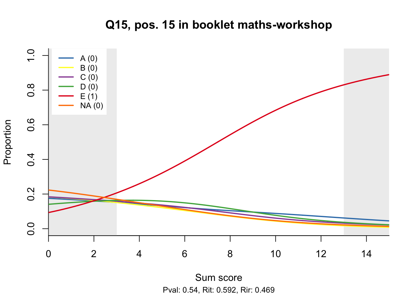
maths-workshop	Q15	0.54	0.50	1	0.54	0.59	0.47	1665
maths-workshop	Q2	0.90	0.30	1	0.90	0.41	0.32	1665
maths-workshop	Q3	0.84	0.37	1	0.84	0.48	0.37	1665
maths-workshop	Q4	0.30	0.46	1	0.30	0.37	0.23	1665
maths-workshop	Q5	0.64	0.48	1	0.64	0.51	0.37	1665
maths-workshop	Q6	0.50	0.50	1	0.50	0.40	0.24	1665
maths-workshop	Q7	0.64	0.48	1	0.64	0.51	0.38	1665
maths-workshop	Q8	0.55	0.50	1	0.55	0.49	0.35	1665
maths-workshop	Q9	0.57	0.50	1	0.57	0.47	0.33	1665

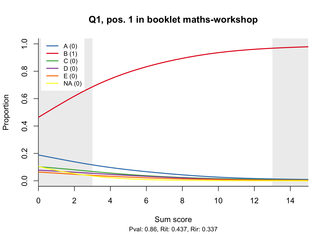
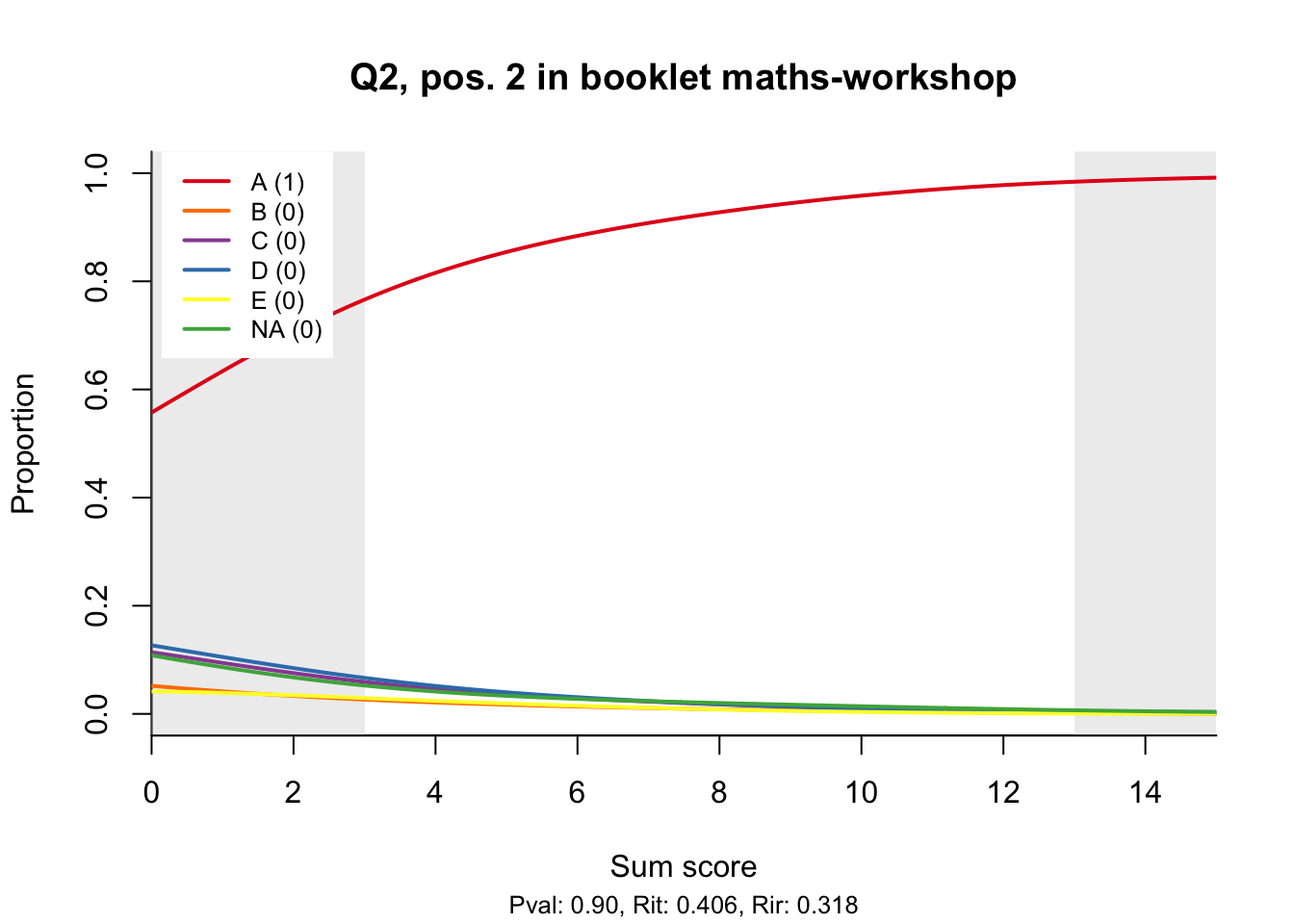
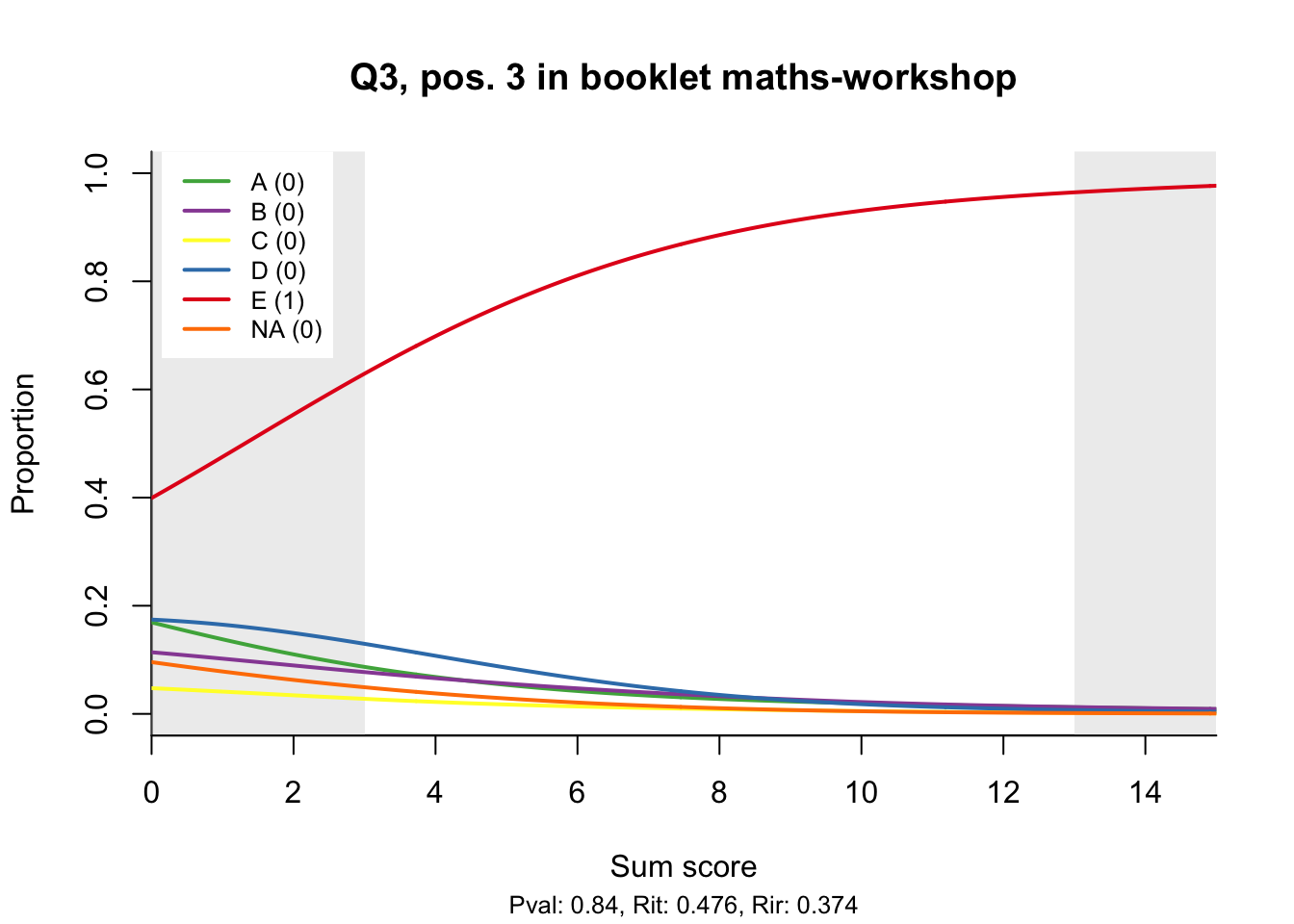
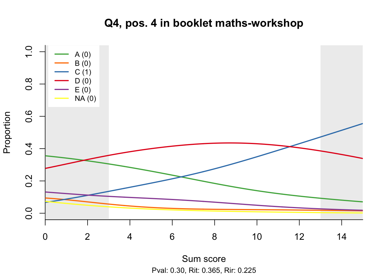
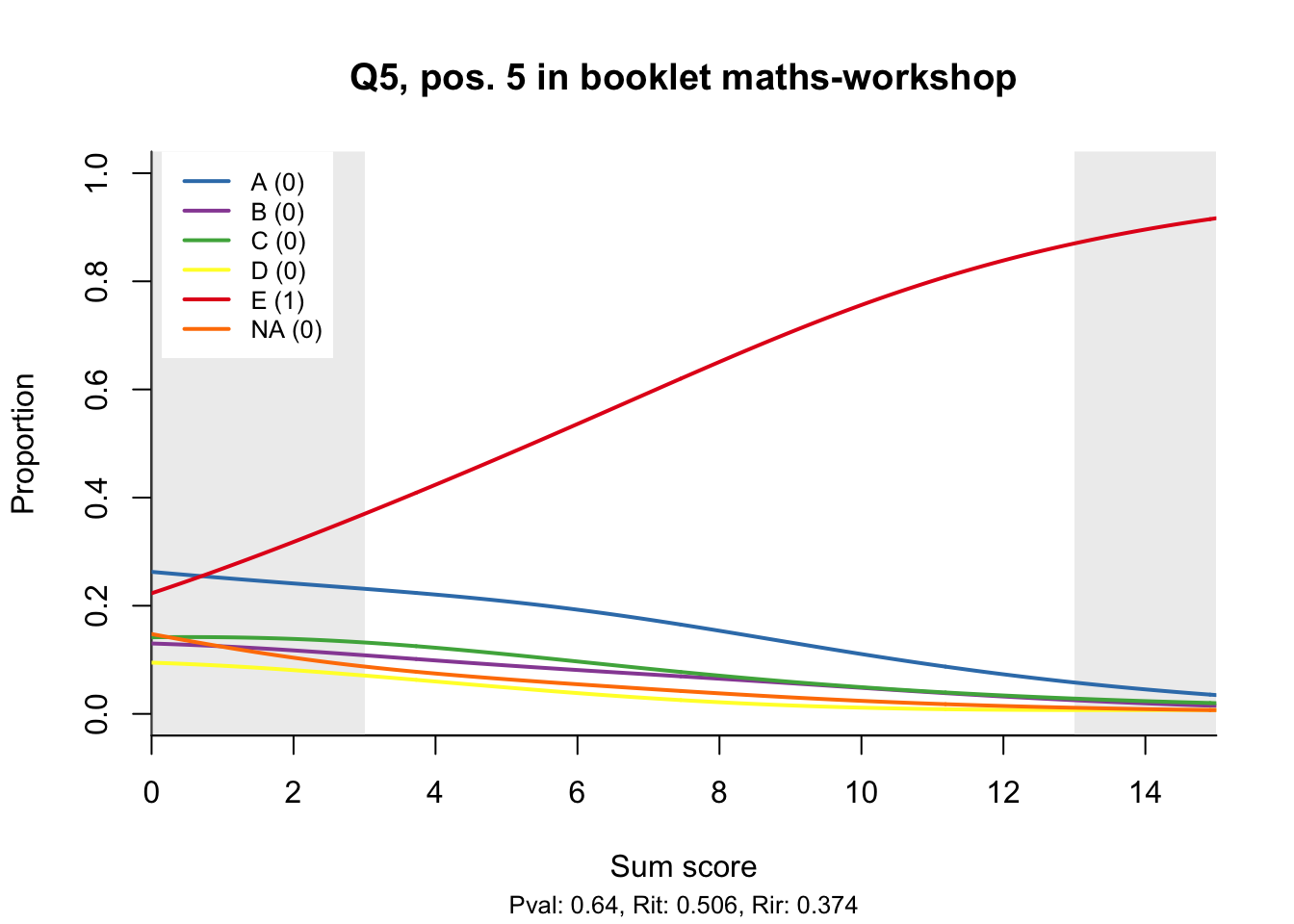
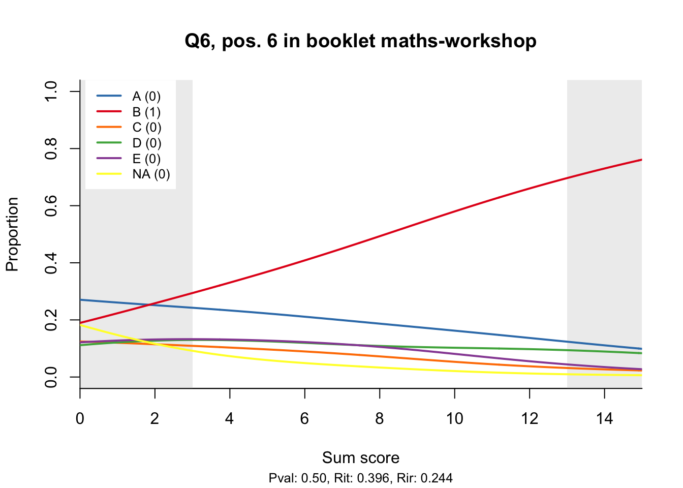
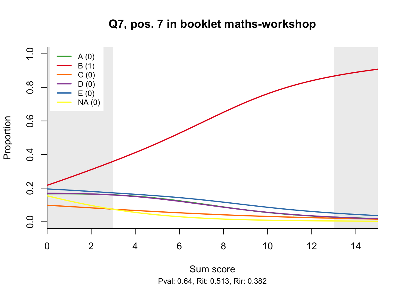
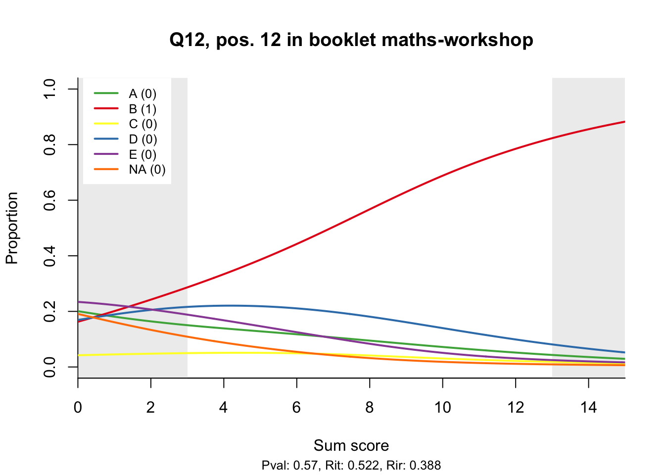
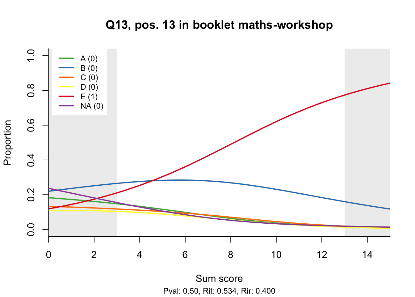
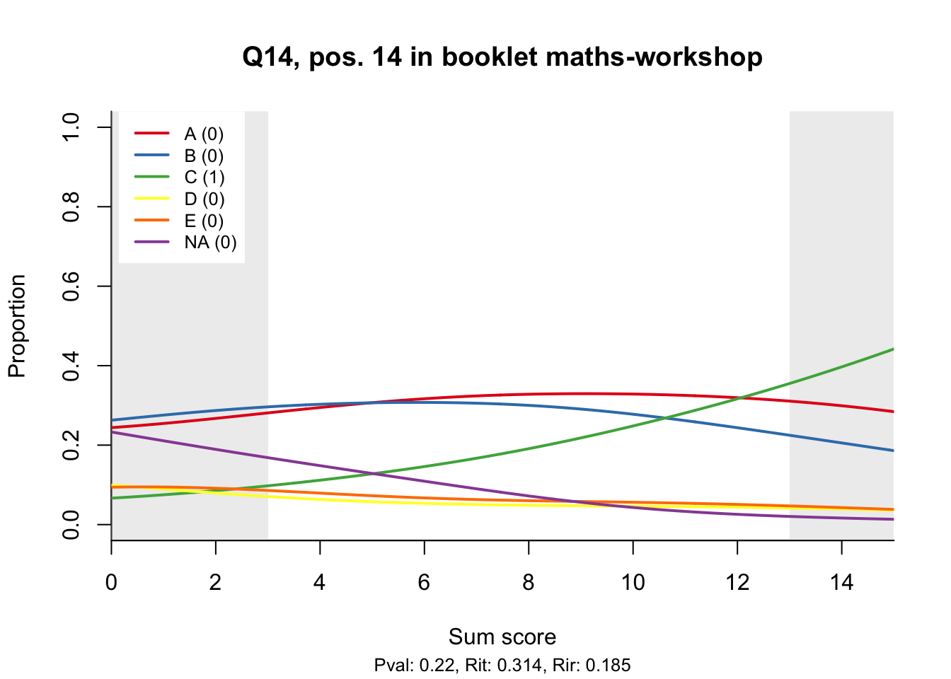
23.3 Distractor analysis

# Look at all the distractor plots
n_items <- nrow(keys)
for(i in 1:n_items){
  distractor_plot(db, keys$item_id[i])
}

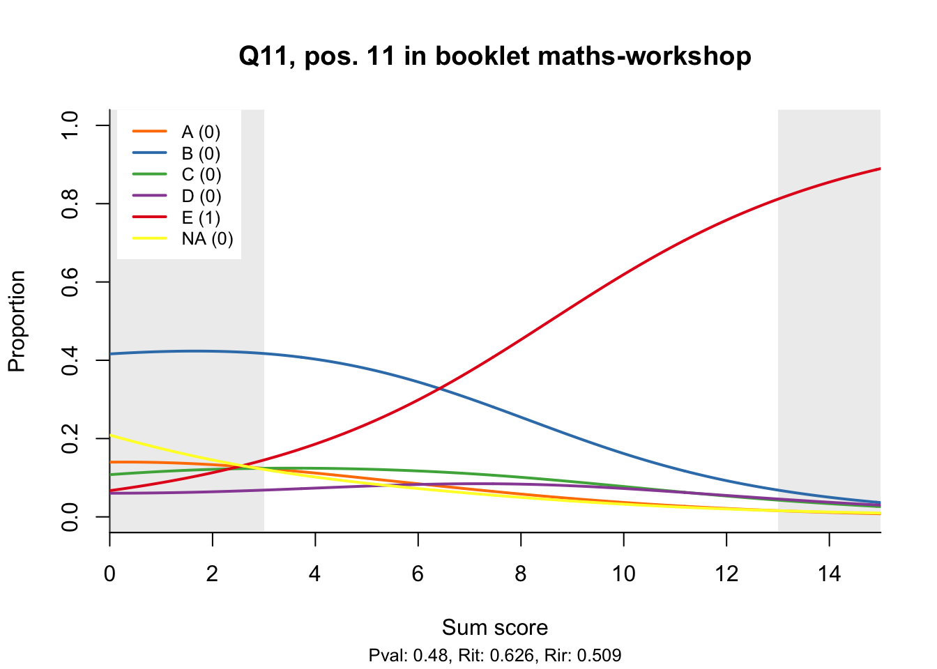
The item test correlations in Table 23.2 suggest an issue with item 10. Let’s look at the distractor plot for that item Figure 23.1.

# produce the distractor plots
# Look at distractor plots for all items
# Something is odd about Q10, so let's look at the distractor plot for that item
distractor_plot(db, 'Q10')

Warning: In density.default(bkl_scores$booklet_score, n = 512, weights = bkl_scores$n/N, 
    adjust = adjust, from = 0, to = max(bkl_scores$booklet_score), 
    warnWbw = FALSE) :
 extra argument 'warnWbw' will be disregarded

Warning: In density.default(.$booklet_score, weights = .$n/sum(.$n), n = 512, 
    bw = dAll$bw, from = min(dAll$x), to = max(dAll$x), warnWbw = FALSE) :
 extra argument 'warnWbw' will be disregarded

Warning: In density.default(.$booklet_score, weights = .$n/sum(.$n), n = 512, 
    bw = dAll$bw, from = min(dAll$x), to = max(dAll$x), warnWbw = FALSE) :
 extra argument 'warnWbw' will be disregarded

Warning: In density.default(.$booklet_score, weights = .$n/sum(.$n), n = 512, 
    bw = dAll$bw, from = min(dAll$x), to = max(dAll$x), warnWbw = FALSE) :
 extra argument 'warnWbw' will be disregarded

Warning: In density.default(.$booklet_score, weights = .$n/sum(.$n), n = 512, 
    bw = dAll$bw, from = min(dAll$x), to = max(dAll$x), warnWbw = FALSE) :
 extra argument 'warnWbw' will be disregarded

Warning: In density.default(.$booklet_score, weights = .$n/sum(.$n), n = 512, 
    bw = dAll$bw, from = min(dAll$x), to = max(dAll$x), warnWbw = FALSE) :
 extra argument 'warnWbw' will be disregarded

Warning: In density.default(.$booklet_score, weights = .$n/sum(.$n), n = 512, 
    bw = dAll$bw, from = min(dAll$x), to = max(dAll$x), warnWbw = FALSE) :
 extra argument 'warnWbw' will be disregarded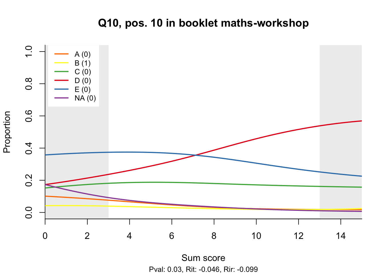

Figure 23.1: Item 10

23.4 Rasch analysis

# run a traditional Rasch analysis using the item scores produced above
library(TAM)
# All the results of the Rasch analysis are stored in the object called "mod1"
mod1 <- TAM::tam.jml(item_scores)
summary(mod1)

knitr::kable(mod1$item1)

Table 23.3: Item Difficulties

xsi.label	xsi.index	xsi	se.xsi
Q1	1	-2.1712756	0.0789443
Q2	2	-2.6145757	0.0903290
Q3	3	-1.9994327	0.0752989
Q4	4	1.0888622	0.0611206
Q5	5	-0.6919299	0.0588426
Q6	6	0.0268089	0.0566208
Q7	7	-0.6757986	0.0587454
Q8	8	-0.2557563	0.0569897
Q9	9	-0.3165510	0.0571532
Q10	10	4.1437076	0.1610654
Q11	11	0.1405420	0.0566530
Q12	12	-0.3135028	0.0571443
Q13	13	0.0268089	0.0566208
Q14	14	1.5975040	0.0670230
Q15	15	-0.1681469	0.0568066

Table 23.4: Item Difficulties Summary

summary(mod1$item1$xsi)

    Min.  1st Qu.   Median     Mean  3rd Qu.     Max. 
-2.61458 -0.68386 -0.25576 -0.14552  0.08367  4.14371 

Table 23.5: Person Abilities Summary

summary(mod1$theta)

    Min.  1st Qu.   Median     Mean  3rd Qu.     Max. 
-5.01490 -0.81791 -0.08508  0.00000  1.14240  5.59084 

library(WrightMap)
wrightMap(mod1$theta, mod1$xsi, item.side = itemClassic)

             [,1]
 [1,] -2.17127562
 [2,] -2.61457572
 [3,] -1.99943270
 [4,]  1.08886221
 [5,] -0.69192988
 [6,]  0.02680892
 [7,] -0.67579856
 [8,] -0.25575627
 [9,] -0.31655103
[10,]  4.14370761
[11,]  0.14054200
[12,] -0.31350278
[13,]  0.02680892
[14,]  1.59750398
[15,] -0.16814688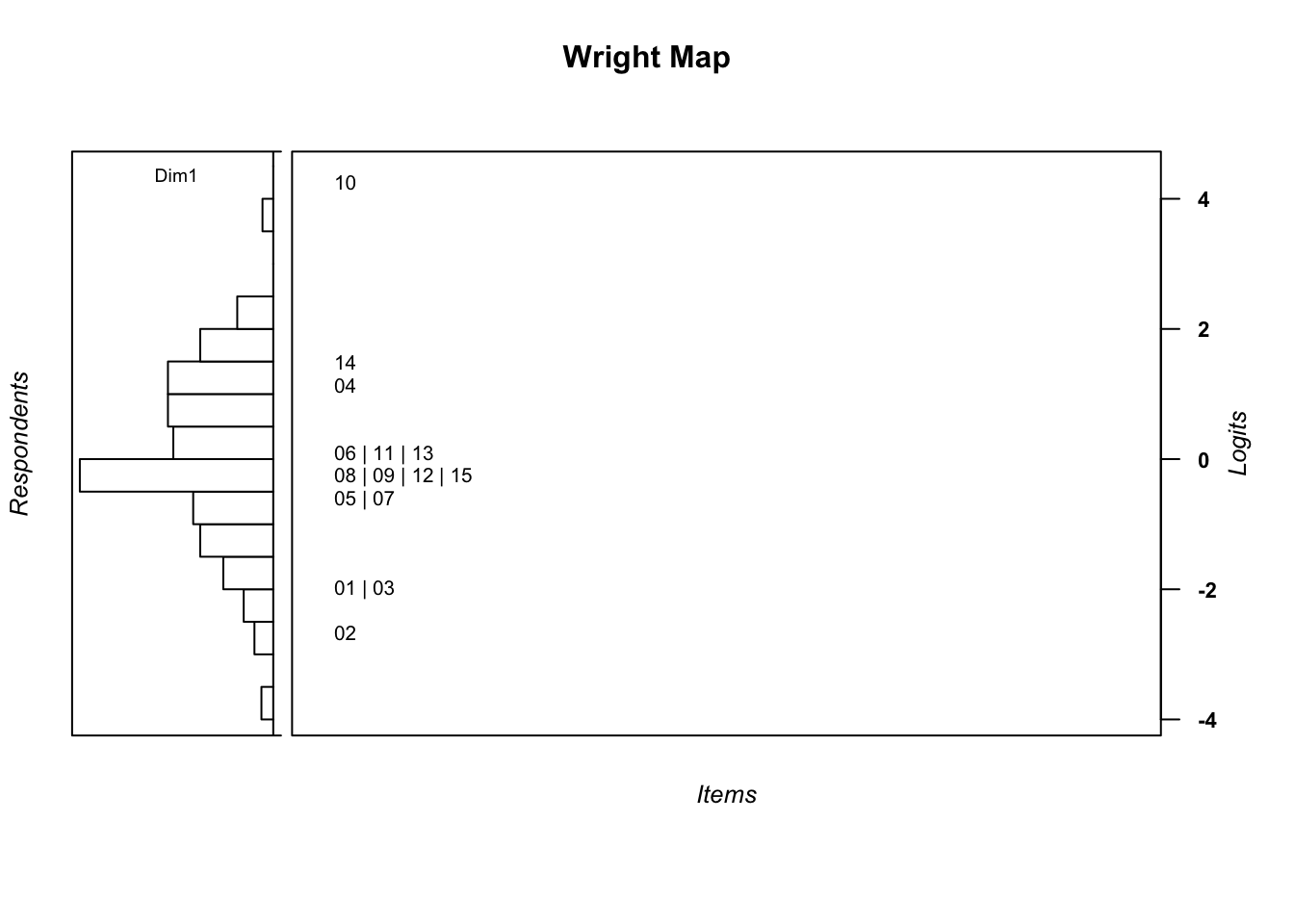

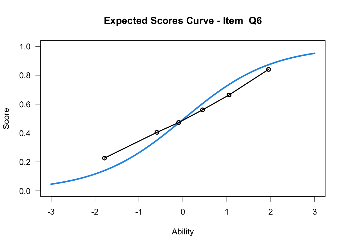
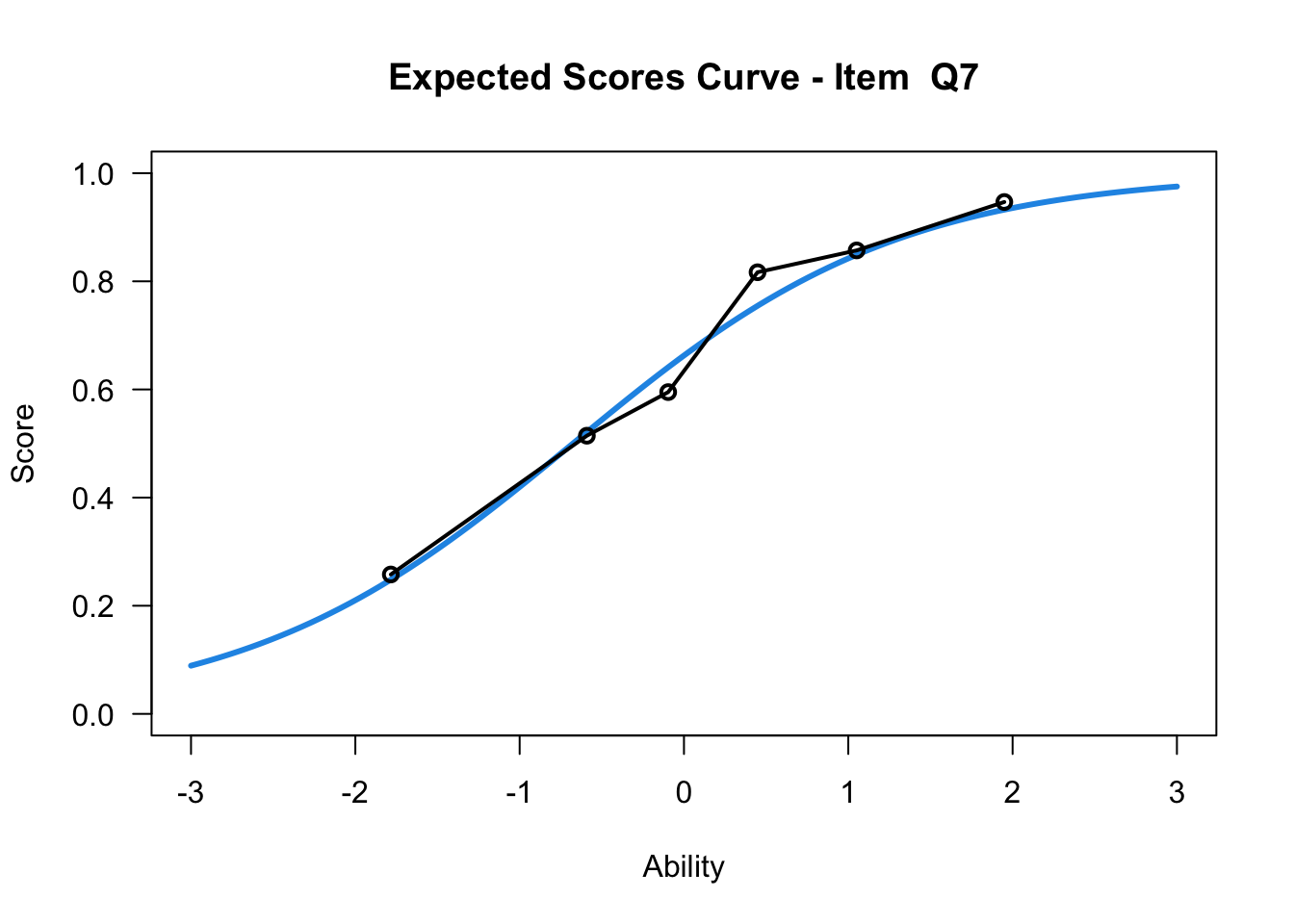
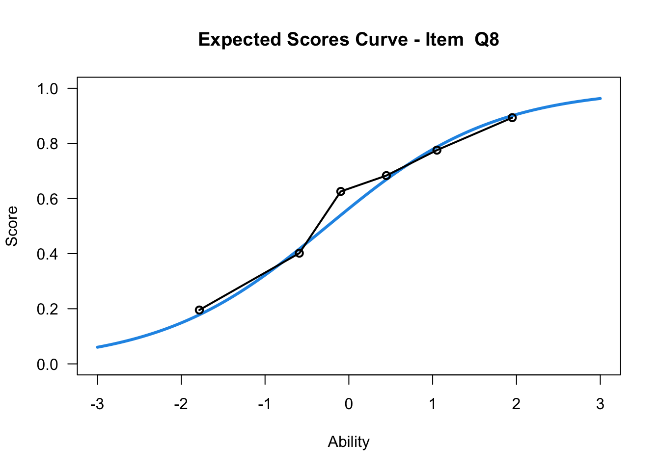
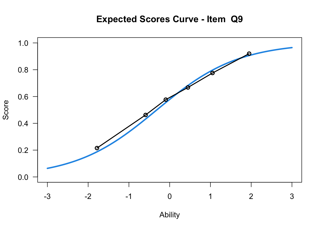
Figure 23.2: Wright Map

plot(mod1,items = c(1:10))

....................................................
 Plots exported in png format into folder:
 /Users/chris/Documents/CM3/Plots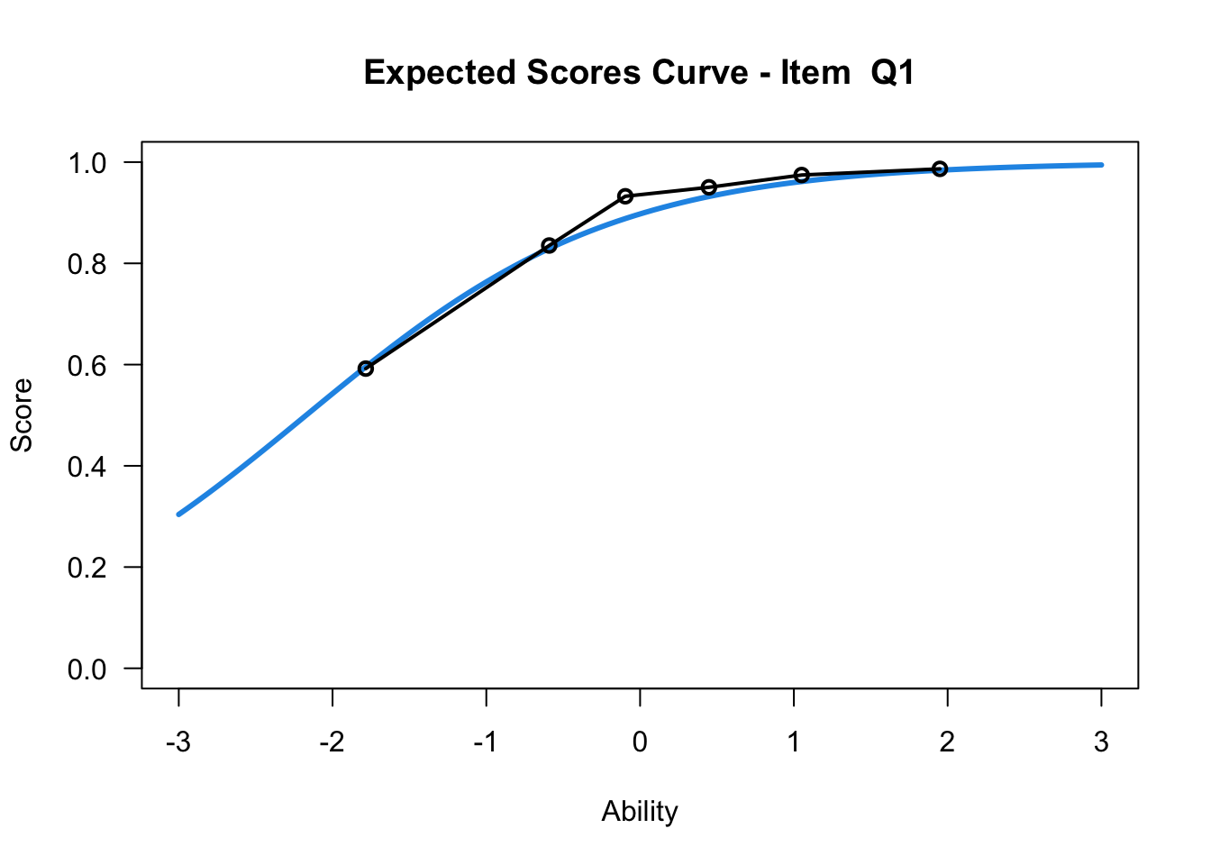

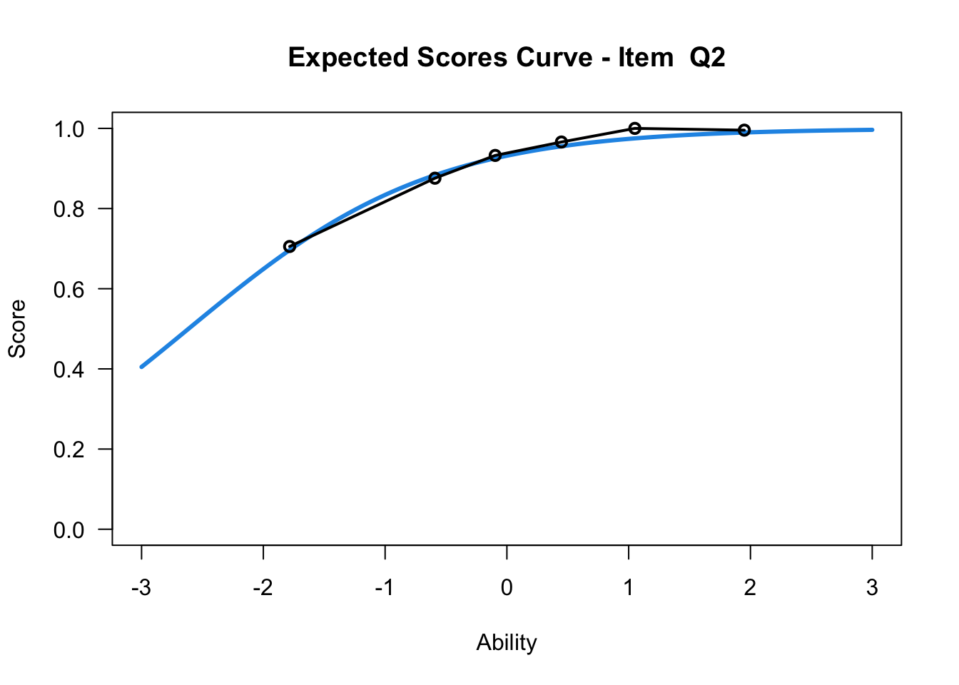
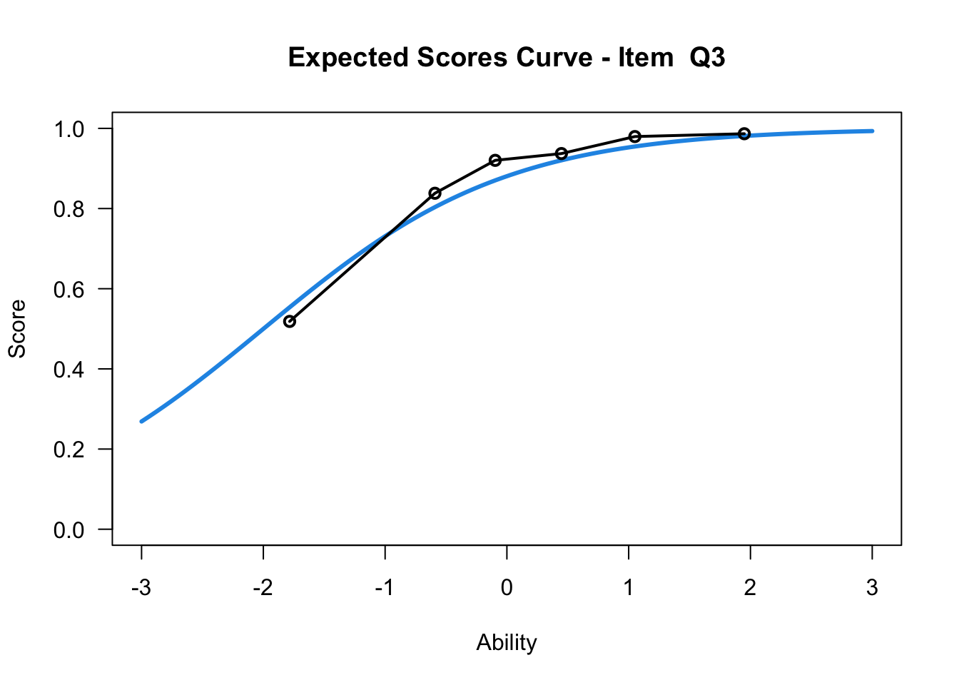
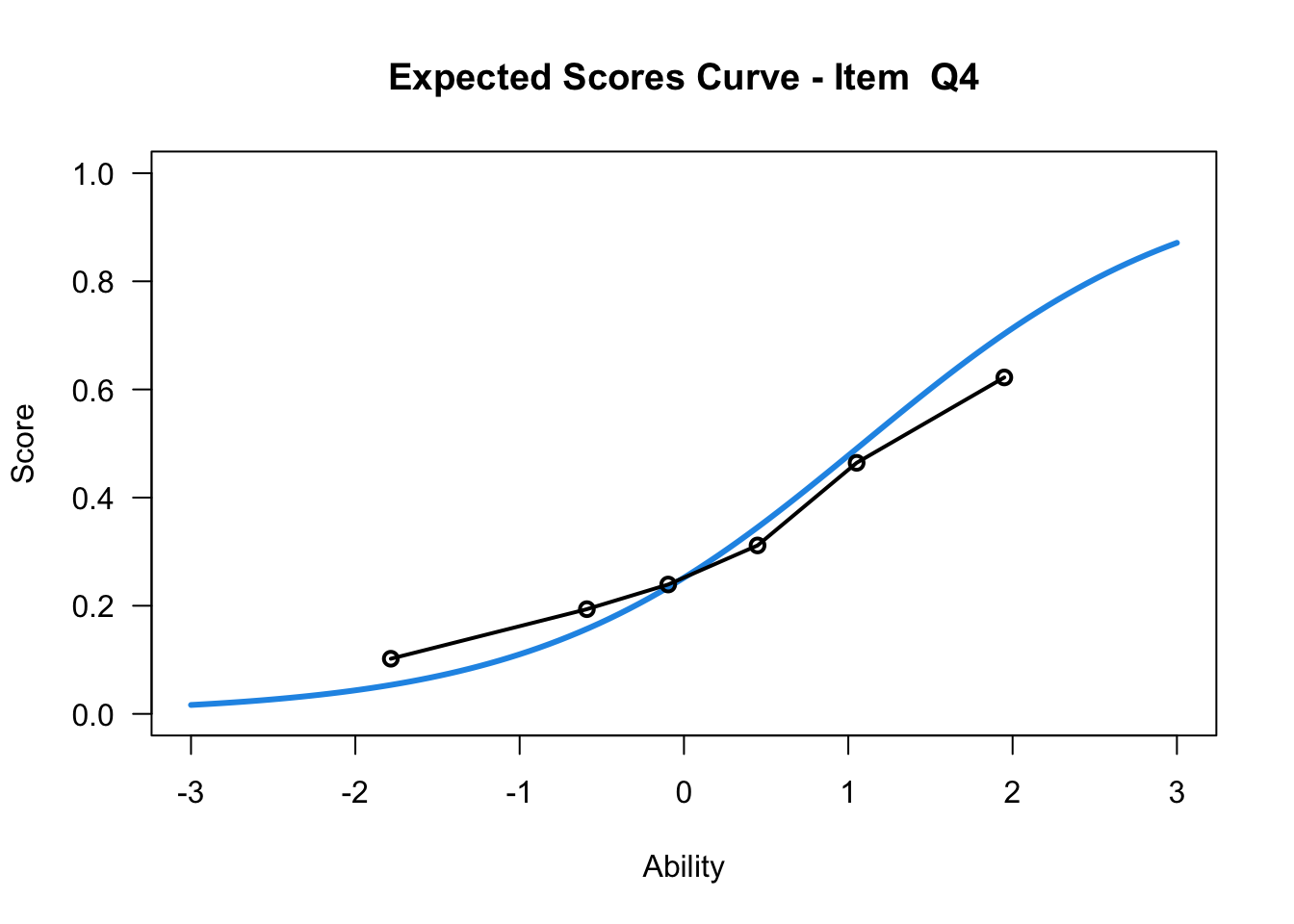
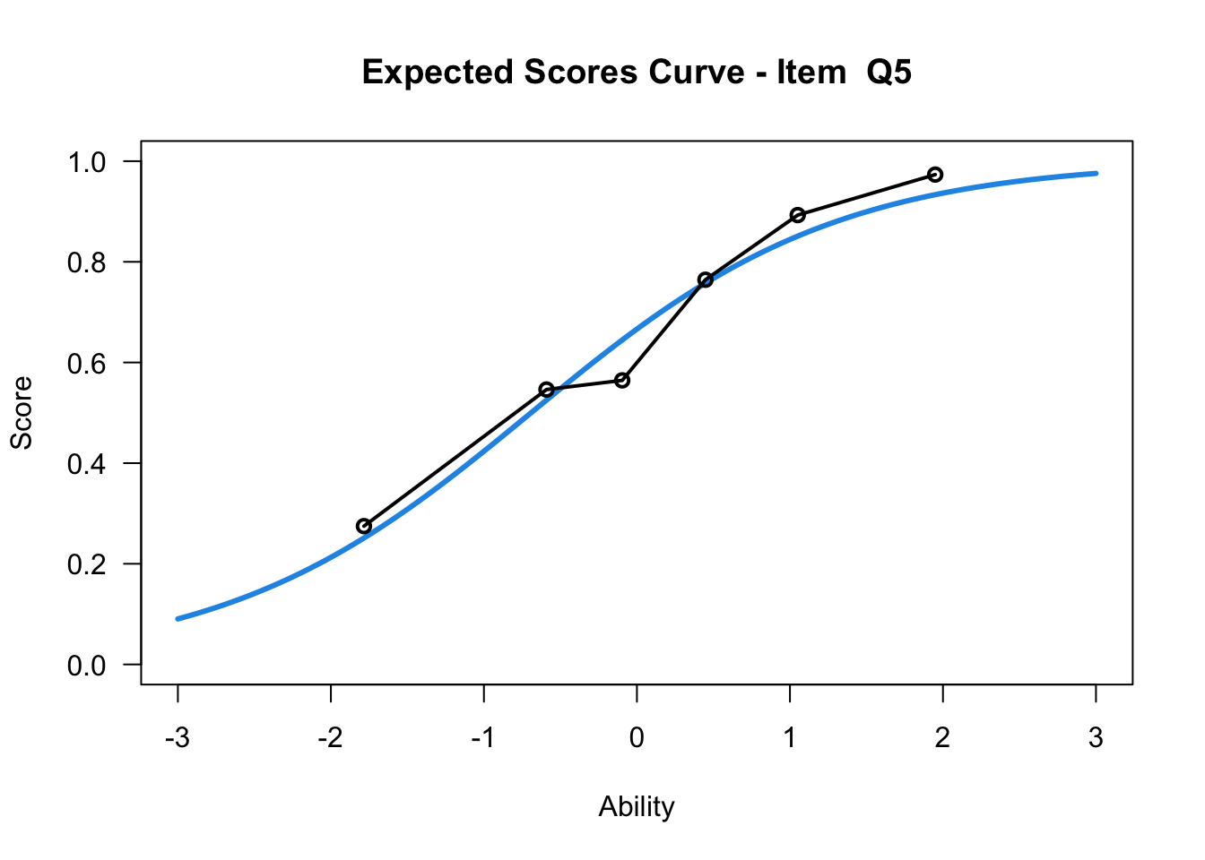
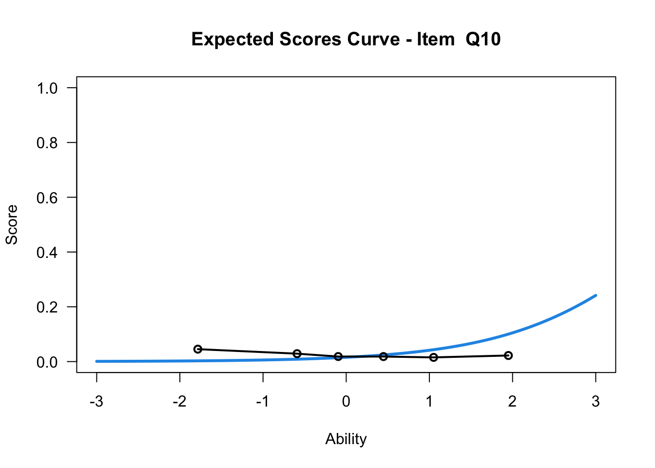
Figure 23.3: ICCs for all items

Figure 23.4: ICCs for all items

Figure 23.5: ICCs for all items

Figure 23.6: ICCs for all items

Figure 23.7: ICCs for all items

Figure 23.8: ICCs for all items

Figure 23.9: ICCs for all items

Figure 23.10: ICCs for all items

Figure 23.11: ICCs for all items

Figure 23.12: ICCs for all items

plot(mod1,items = c(10))

....................................................
 Plots exported in png format into folder:
 /Users/chris/Documents/CM3/Plots

Figure 23.13: ICC for Q10

fit1 <- tam.jml.fit(mod1,trim_val = NULL)
item_fit <- tibble(fit1$fit.item)
item_fit <- item_fit %>% bind_cols(mod1$item1)
knitr::kable(item_fit, digits = 2)

item	outfitItem	outfitItem_t	infitItem	infitItem_t	xsi.label	xsi.index	xsi	se.xsi
Q1	0.81	-1.66	0.88	-2.58	Q1	1	-2.17	0.08
Q2	0.70	-2.24	0.86	-2.63	Q2	2	-2.61	0.09
Q3	0.77	-2.26	0.86	-3.51	Q3	3	-2.00	0.08
Q4	1.16	2.11	1.09	3.23	Q4	4	1.09	0.06
Q5	0.92	-1.37	0.98	-0.76	Q5	5	-0.69	0.06
Q6	1.21	3.84	1.14	5.78	Q6	6	0.03	0.06
Q7	0.91	-1.55	0.97	-1.23	Q7	7	-0.68	0.06
Q8	1.00	0.06	1.01	0.44	Q8	8	-0.26	0.06
Q9	1.04	0.75	1.04	1.65	Q9	9	-0.32	0.06
Q10	5.43	6.42	0.95	-0.35	Q10	10	4.14	0.16
Q11	0.74	-5.57	0.81	-8.65	Q11	11	0.14	0.06
Q12	0.91	-1.78	0.97	-1.34	Q12	12	-0.31	0.06
Q13	0.92	-1.55	0.95	-2.31	Q13	13	0.03	0.06
Q14	1.43	3.96	1.06	1.85	Q14	14	1.60	0.07
Q15	0.80	-4.19	0.87	-5.75	Q15	15	-0.17	0.06

Item Fit Statistics

# plot the item infit against the item difficulty
p <- ggplot(item_fit, aes(x=infitItem, y=xsi, size=se.xsi,label=item))
p <- p + geom_point()
p <- p + geom_text(data=item_fit %>% filter(infitItem>1.1),aes(x=infitItem, y=xsi,label=item,size=4),nudge_y=0.15, nudge_x = -0.005)
print(p)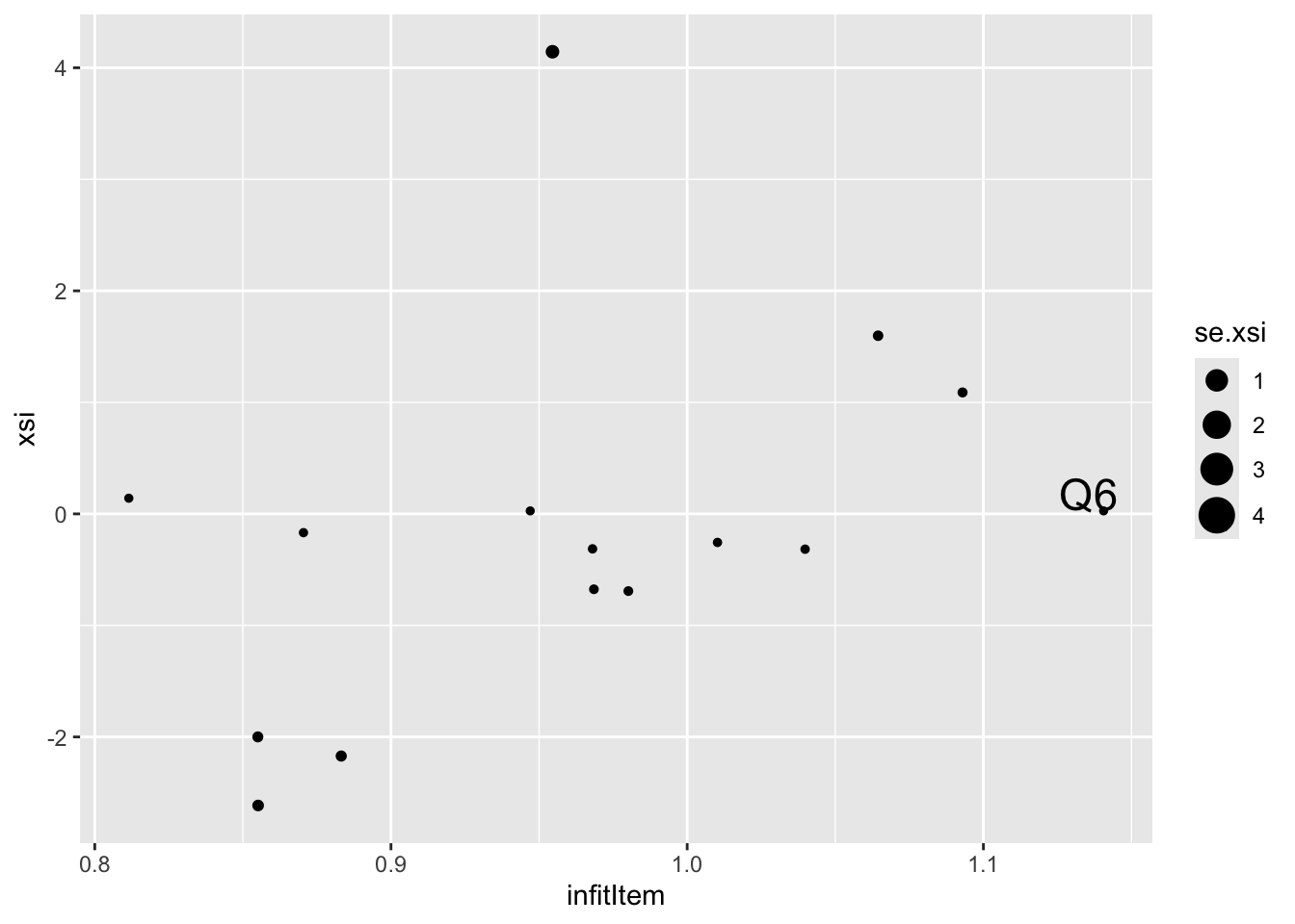

Figure 23.14: Rasch Bubble Plot

# plot the item outfit against the item difficulty
p <- ggplot(item_fit, aes(x=outfitItem, y=xsi, size=se.xsi,label=item))
p <- p + geom_point()
p <- p + geom_text(data=item_fit %>% filter(outfitItem>1.1),aes(x=outfitItem, y=xsi,label=item,size=4),nudge_y=0.15, nudge_x = -0.005)
print(p)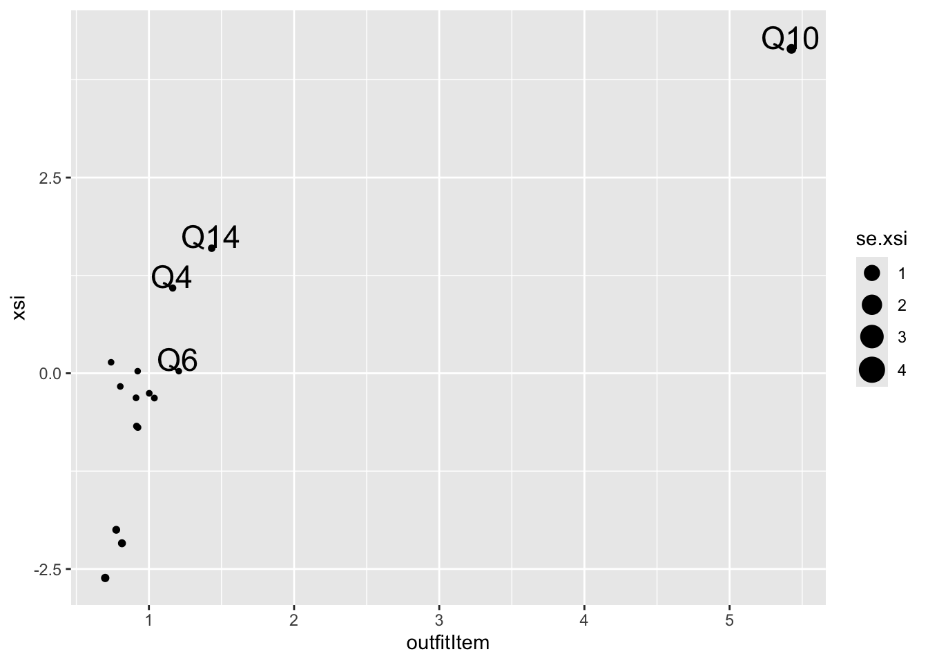

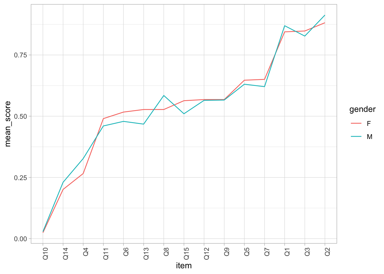
Figure 23.15: Rasch Bubble Plot Using Outfit

23.5 DIF

item_scores <- item_scores %>% mutate(gender = responses$gender)
long_responses <- item_scores %>% pivot_longer(cols = Q1:Q15, names_to = "question", values_to = "score")
long_responses <- long_responses %>% mutate(gender = factor(gender))
long_responses <- long_responses %>% mutate(question = factor(question))

response_summary <- long_responses %>% 
  group_by(gender, question) %>%
  summarise(mean_score = mean(score,na.rm=TRUE))

`summarise()` has grouped output by 'gender'. You can override using the
`.groups` argument.

question_difficulty <- response_summary %>%
  filter(gender=='F') %>% 
  arrange(mean_score) %>% pull(question)

ordered_responses <- response_summary %>% mutate(item = factor(question, levels=question_difficulty, ordered=TRUE))
ordered_responses <- ordered_responses %>% mutate(
  gender = factor(gender)
)

p <- ggplot(ordered_responses, aes(x=item, y=mean_score, group=gender, colour=gender, line_style=gender))
p <- p + geom_line() # rotate the x-axis labels
p <- p + theme_light()
p <- p + theme(axis.text.x = element_text(angle = 90, hjust = 1))
p

Figure 23.16: DIF using proportion correct

Andrich, David, and Ida Marais. 2019. “The Idea of Measurement.” In A Course in Rasch Measurement Theory, 3–11. Springer Nature Singapore. https://doi.org/10.1007/978-981-13-7496-8_1.

Bond, Trevor G., Zi Yan, and Moritz Heene. 2020. Applying the Rasch Model: Fundamental Measurement in the Human Sciences. Routledge. https://doi.org/10.4324/9780429030499.

Cappelleri, Jason Lundy, J. C. 2014. “Overview of Classical Test Theory and Item Response Theory for the Quantitative Assessment of Items in Developing Patient-Reported Outcomes Measures.” Clinical Therapeutics 36 (5): 648–62. https://doi.org/https://doi.org/10.1016/j.clinthera.2014.04.006.

Cronbach, Lee J. 1951. “Coefficient Alpha and the Internal Structure of Tests.” Psychometrika 16 (3): 297–334. https://doi.org/10.1007/bf02310555.

Goldstein, H., and Steve Blinkhorn. 1982. “The Rasch Model Still Does Not Fit.” British Educational Research Journal 8 (2): 167–70. https://doi.org/10.1080/0141192820080207.

Lord, Frederic M, and Melvin R Novick. 2008. Statistical Theories of Mental Test Scores. IAP.

McNeish, Daniel. 2018. “Thanks Coefficient Alpha, We’ll Take It from Here.” Psychological Methods 23 (3): 412–33. https://doi.org/10.1037/met0000144.

Panayides, Panayiotis, Colin Robinson, and Peter Tymms. 2010. “The Assessment Revolution That Has Passed England by: Rasch Measurement.” British Educational Research Journal 36 (4): 611–26. https://doi.org/10.1080/01411920903018182.

Robitzsch, Alexander, Thomas Kiefer, and Margaret Wu. 2022. TAM: Test Analysis Modules. https://CRAN.R-project.org/package=TAM.

Sijtsma, Klaas. 2008. “On the Use, the Misuse, and the Very Limited Usefulness of Cronbach’s Alpha.” Psychometrika 74 (1): 107–20. https://doi.org/10.1007/s11336-008-9101-0.

Wright, Benjamin D, and Magdalena Mok. 2000. “Rasch Models Overview.” Journal of Applied Measurement 1 (1): 83–106.