24 What is the Partial Credit Model?
When test items are scored with partial credit scores such as 0, 1 or 2, and not just as correct or incorrect, the model is called the partial credit model (PCM) Equation 24.1
\[ Prob(X=0) = \frac{1}{1+\exp(\theta - \delta_1) + \exp(2\theta - \delta_1 - \delta_2)} \tag{24.1}\] \[ Prob(X=1) = \frac{\exp(\theta - \delta_1)}{1+\exp(\theta - \delta_1) + \exp(2\theta - \delta_1 - \delta_2)} \tag{24.2}\] \[ Prob(X=2) = \frac{\exp(2\theta - \delta_1 - \delta_2)}{1+\exp(\theta - \delta_1) + \exp(2\theta - \delta_1 - \delta_2)} \tag{24.3}\]
where θ is the ability parameter, and δ1 and δ2 are two item difficulty parameters for this item. Note that the denominator is just the sum of the numerators, so the probabilities add up to one.
24.1 Interpretations of the PCM Andrich item thresholds
In the dichotomous case, the item difficulty parameter, δ, is the ability measure at which students have 50% chance of obtaining the correct answer for the item. That is, the item difficulty is the ability measure at which the chance of obtaining a 0 or 1 is the same. In the partial credit model, the δ values are the ability measures at which persons have an equal chance of being in two adjacent scoring categories. With three score categories, we need two thresholds, δ1 and δ2. Let’s set δ1 = -0.5 and δ2 = 1.7. So -0.5 (δ1) is the ability at which a person has an equal chance of being in category 0 or category 1. Similarly, 1.7 (δ2) is the ability at which a person has an equal chance of being in category 1 or category 2.
24.2 Let’s calculate some probabilities
Using our two category parameters, δ1 and δ2 at -0.5 and 1.7 we can calculate the probabilities of a person of ability 0, scoring 0 as follows:
\[ Prob(X=0) = \frac{1}{1+\exp(0 +0.5) + \exp(0 +0.5 -1.7)} \tag{24.4}\]
\[ Prob(X=0) = \frac{1}{1+1.648721 + 3.320117} \tag{24.5}\]
\[ Prob(X=0) = \frac{1}{0.1675368} \tag{24.6}\]
\[ Prob(X=0) = 0.3389928 \tag{24.7}\]
Now calculate the probabilities for the other two score categories.
24.3 Visualising the Item Characteristic Curves of our PCM item
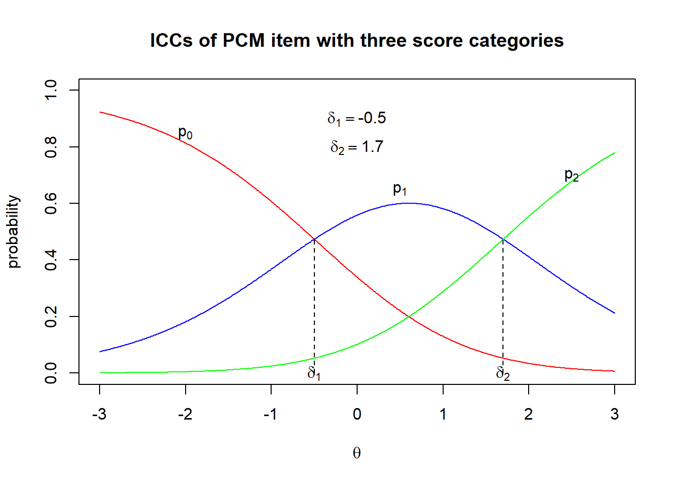
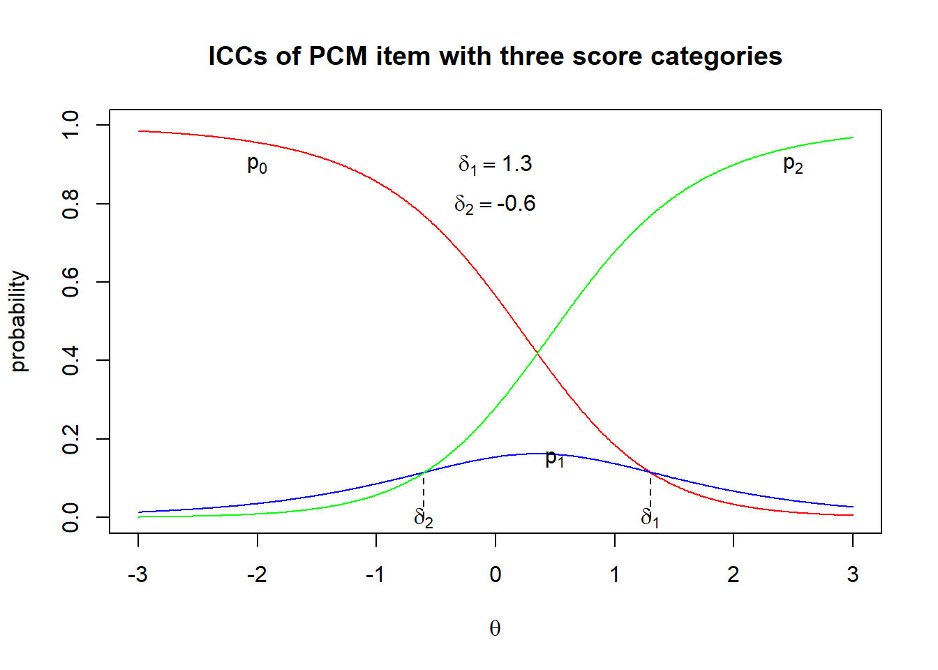
Figure 24.1 and Figure 24.2 show the item characteristic curves for two PCM items, plotted according to Equation 24.1, Equation 24.2 and Equation 24.3.
It can be seen in both figures that δ1 is the intersection point of p0 and p1, showing the ability at which the two probabilities are equal. Similarly, δ2 is the intersection point of p1 and p2, where the probability of obtaining a score of 1 is the same as the probability of obtaining a score of 2. However, in Figure 24.1 ,δ1 is smaller than δ2, whereas in Figure Figure 24.2, δ1 is greater than δ2 . This common phenomenon is known as disordered thresholds. Disordered thresholds occur when a middle score category (score of 1 in this case) has few students as reflected in the low p1 curve. Disordered thresholds do not indicate that the item is problematic, it just means that students are most likely to obtain 0 or 2, and few students would obtain a score of 1.
It is important to note that the thresholds do not represent the difficulty of an item, simply the crossover points between categories. It is misleading to compare thresholds between items when analysing the relative difficulty of items.
24.4 Extension task
From the equations, see if you can create the curves in Figure 24.1 and Figure 24.2.
24.5 Further Reading
http://www.edmeasurementsurveys.com/IRT/partial-credit-models---part-i.html