27  Fitting the Partial Credit Model

You can fit the Partial Credit Model in either dexter or TAM. Let’s start with dexter.

rm(list=ls())
library(tidyverse)
library(dexter)
# load in the dataset
responses <- read_csv('data/pc-data.csv')
# recode NA as 0 across all columns
responses <- responses %>% 
  mutate_if(is.numeric, ~replace_na(., 0))
# load the data summary
data_summary <- read_csv('data/pc-data-summary.csv')

# Create the rules from the summary
# create an empty tibble with three columns item_id, response, and item_score
rules <- tibble(item_id = character(), response = character(), item_score = numeric())

# for each row in the data summary create a rule
for (i in 1:nrow(data_summary)) {
  # get the item id
  item_id <- data_summary$Variable[i]
  # get the maximum mark
  max_mark <- data_summary$`Maximum possible mark`[i]
  # for every mark from 0 to max_mark create a rule
    for (mark in 0:max_mark) {
        # create a rule for the mark
        rule <- tibble(item_id = item_id, response = as.character(mark), item_score = mark)
        # add the rule to the rules tibble
        rules <- bind_rows(rules, rule)
    }
}

# create a new project
db <- start_new_project(rules, db_name = ":memory:", person_properties=list(sex="unknown",grade="unknown"))
# add the response data
add_booklet(db, responses, "geography")

no column `person_id` provided, automatically generating unique person id's

$items
 [1] "C1_1ai"    "C1_1aii"   "C1_1bi"    "C1_1bii"   "C1_1biii"  "C1_1biv"  
 [7] "C1_1ci"    "C1_1cii"   "C1_1di"    "C1_1dii"   "C1_1e"     "C1_1eSPaG"
[13] "C1_2ai"    "C1_2aii"   "C1_2bi"    "C1_2bii"   "C1_2biii"  "C1_2biv"  
[19] "C1_2bv"    "C1_2c"     "C1_2d"     "C1_3ai"    "C1_3aii"   "C1_3aiii" 
[25] "C1_3bi"    "C1_3bii"   "C1_3ci"    "C1_3cii"   "C1_3d"     "C2_Aa"    
[31] "C2_Ab"     "C2_Ac"     "C2_Adi"    "C2_Adii"   "C2_Aei"    "C2_Aeii"  
[37] "C2_Aeiii"  "C2_Aeiv"   "C2_Af"     "C2_Ag"     "C2_Bai"    "C2_Baii"  
[43] "C2_Bb"     "C2_Bc"     "C2_Bd"     "C2_Be"     "C2_Bf"     "C2_C"     
[49] "C2_CSPaG"  "C3_1ai"    "C3_1aii"   "C3_1bi"    "C3_1bii"   "C3_1biii" 
[55] "C3_1c"     "C3_2ai"    "C3_2aii"   "C3_2b"     "C3_2ci"    "C3_2cii"  
[61] "C3_2ciii"  "C3_2d"     "C3_3ai"    "C3_3aii"   "C3_3aiii"  "C3_3b"    
[67] "C3_3ci"    "C3_3cii"   "C3_3di"    "C3_3dii"   "C3_3e"     "C3_3f"    
[73] "C3_3fSPaG"

$person_properties
[1] "sex"   "grade"

$columns_ignored
[1] "C1_total" "C2_total" "C3_total" "total"   

# print the item tables
tt = tia_tables(db)
knitr::kable(tt$items, digits=2)

booklet_id	item_id	mean_score	sd_score	max_score	pvalue	rit	rir	n_persons
geography	C1_1ai	0.96	0.18	1	0.96	0.24	0.24	8500
geography	C1_1aii	2.72	0.51	3	0.91	0.38	0.37	8500
geography	C1_1bi	0.97	0.18	1	0.97	0.20	0.19	8500
geography	C1_1bii	0.71	0.45	1	0.71	0.34	0.33	8500
geography	C1_1biii	0.98	0.78	2	0.49	0.43	0.41	8500
geography	C1_1biv	0.53	0.50	1	0.53	0.49	0.48	8500
geography	C1_1ci	0.91	1.12	4	0.23	0.46	0.44	8500
geography	C1_1cii	2.50	1.40	6	0.42	0.61	0.58	8500
geography	C1_1di	1.63	1.08	3	0.54	0.44	0.42	8500
geography	C1_1dii	1.09	0.81	2	0.54	0.49	0.47	8500
geography	C1_1e	3.75	1.73	8	0.47	0.69	0.67	8500
geography	C1_1eSPaG	2.69	0.80	4	0.67	0.60	0.59	8500
geography	C1_2ai	2.85	1.28	4	0.71	0.49	0.46	8500
geography	C1_2aii	3.12	0.92	4	0.78	0.35	0.32	8500
geography	C1_2bi	0.85	0.36	1	0.85	0.36	0.35	8500
geography	C1_2bii	1.43	0.84	2	0.71	0.46	0.44	8500
geography	C1_2biii	2.61	0.62	3	0.87	0.38	0.37	8500
geography	C1_2biv	1.15	0.95	2	0.58	0.57	0.55	8500
geography	C1_2bv	0.65	0.85	2	0.33	0.50	0.49	8500
geography	C1_2c	2.36	2.01	6	0.39	0.68	0.65	8500
geography	C1_2d	3.34	1.65	8	0.42	0.67	0.65	8500
geography	C1_3ai	2.90	1.16	4	0.72	0.65	0.64	8500
geography	C1_3aii	0.96	0.73	2	0.48	0.37	0.36	8500
geography	C1_3aiii	1.41	1.19	4	0.35	0.54	0.51	8500
geography	C1_3bi	0.92	0.28	1	0.92	0.28	0.28	8500
geography	C1_3bii	1.57	1.18	4	0.39	0.54	0.51	8500
geography	C1_3ci	2.24	0.96	3	0.75	0.60	0.58	8500
geography	C1_3cii	2.68	1.72	6	0.45	0.70	0.67	8500
geography	C1_3d	3.36	1.70	8	0.42	0.68	0.66	8500
geography	C2_Aa	2.34	1.27	5	0.47	0.40	0.37	8500
geography	C2_Ab	1.75	1.18	4	0.44	0.41	0.39	8500
geography	C2_Ac	2.83	1.15	4	0.71	0.56	0.54	8500
geography	C2_Adi	3.31	1.03	4	0.83	0.50	0.48	8500
geography	C2_Adii	1.42	0.93	3	0.47	0.51	0.50	8500
geography	C2_Aei	0.94	0.24	1	0.94	0.21	0.21	8500
geography	C2_Aeii	1.92	1.05	3	0.64	0.64	0.63	8500
geography	C2_Aeiii	0.78	0.85	4	0.20	0.41	0.40	8500
geography	C2_Aeiv	0.55	0.67	2	0.28	0.26	0.25	8500
geography	C2_Af	1.48	0.81	3	0.49	0.46	0.44	8500
geography	C2_Ag	3.17	1.52	6	0.53	0.66	0.64	8500
geography	C2_Bai	0.90	0.30	1	0.90	0.33	0.32	8500
geography	C2_Baii	0.77	0.57	2	0.38	0.49	0.48	8500
geography	C2_Bb	1.25	1.23	4	0.31	0.43	0.41	8500
geography	C2_Bc	1.11	0.75	2	0.56	0.40	0.39	8500
geography	C2_Bd	2.67	1.39	5	0.53	0.65	0.63	8500
geography	C2_Be	2.30	1.43	4	0.58	0.59	0.56	8500
geography	C2_Bf	1.21	0.97	3	0.40	0.50	0.49	8500
geography	C2_C	6.69	3.23	12	0.56	0.77	0.73	8500
geography	C2_CSPaG	2.95	1.06	4	0.74	0.70	0.69	8500
geography	C3_1ai	0.42	0.63	2	0.21	0.46	0.45	8500
geography	C3_1aii	1.70	0.61	2	0.85	0.44	0.42	8500
geography	C3_1bi	1.60	0.77	2	0.80	0.51	0.50	8500
geography	C3_1bii	0.72	0.74	2	0.36	0.46	0.44	8500
geography	C3_1biii	1.34	1.16	4	0.33	0.60	0.58	8500
geography	C3_1c	1.54	1.57	6	0.26	0.60	0.57	8500
geography	C3_2ai	1.64	0.59	2	0.82	0.16	0.15	8500
geography	C3_2aii	1.27	0.98	4	0.32	0.49	0.48	8500
geography	C3_2b	1.56	0.59	2	0.78	0.41	0.40	8500
geography	C3_2ci	0.77	0.42	1	0.77	0.37	0.36	8500
geography	C3_2cii	0.95	0.22	1	0.95	0.27	0.26	8500
geography	C3_2ciii	1.47	0.96	4	0.37	0.54	0.52	8500
geography	C3_2d	1.37	1.15	4	0.34	0.61	0.59	8500
geography	C3_3ai	2.43	0.75	3	0.81	0.50	0.48	8500
geography	C3_3aii	1.90	0.37	2	0.95	0.39	0.38	8500
geography	C3_3aiii	2.78	1.19	4	0.69	0.67	0.65	8500
geography	C3_3b	0.79	0.41	1	0.79	0.37	0.36	8500
geography	C3_3ci	1.39	0.87	2	0.70	0.42	0.40	8500
geography	C3_3cii	1.81	0.50	2	0.91	0.42	0.41	8500
geography	C3_3di	0.26	0.44	1	0.26	0.23	0.22	8500
geography	C3_3dii	2.29	1.58	6	0.38	0.62	0.59	8500
geography	C3_3e	0.95	0.81	3	0.32	0.44	0.43	8500
geography	C3_3f	5.55	2.64	12	0.46	0.75	0.72	8500
geography	C3_3fSPaG	2.88	1.05	4	0.72	0.64	0.62	8500

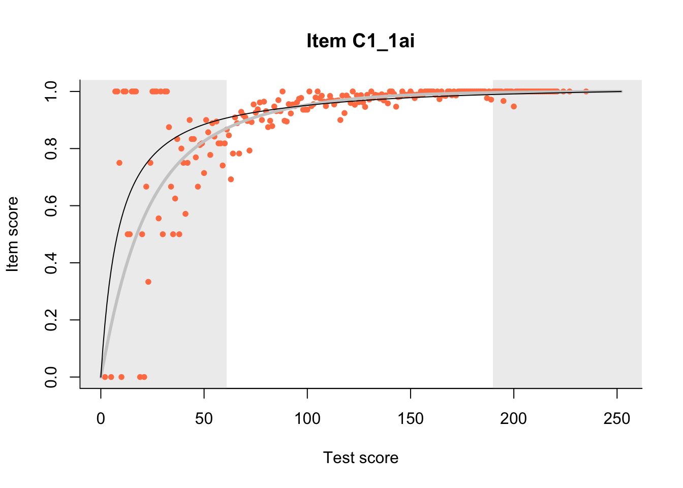
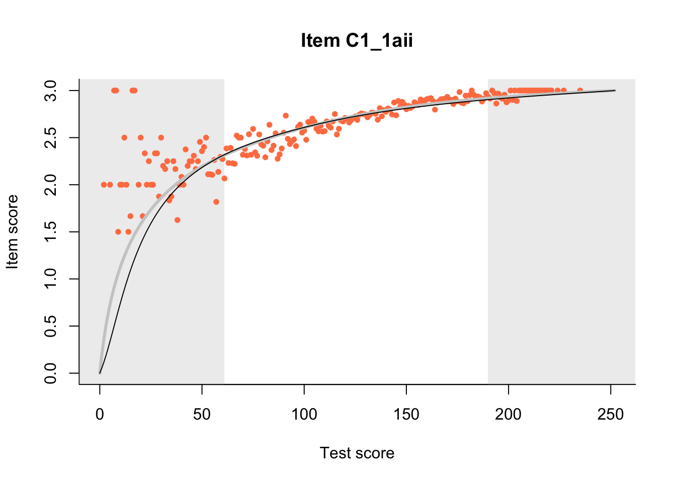
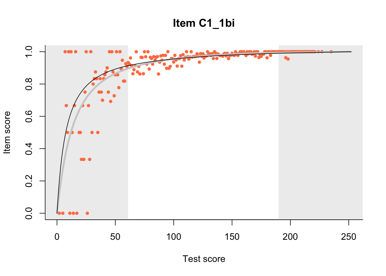
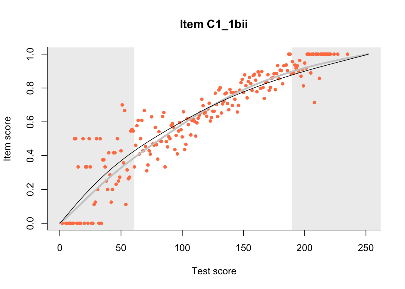
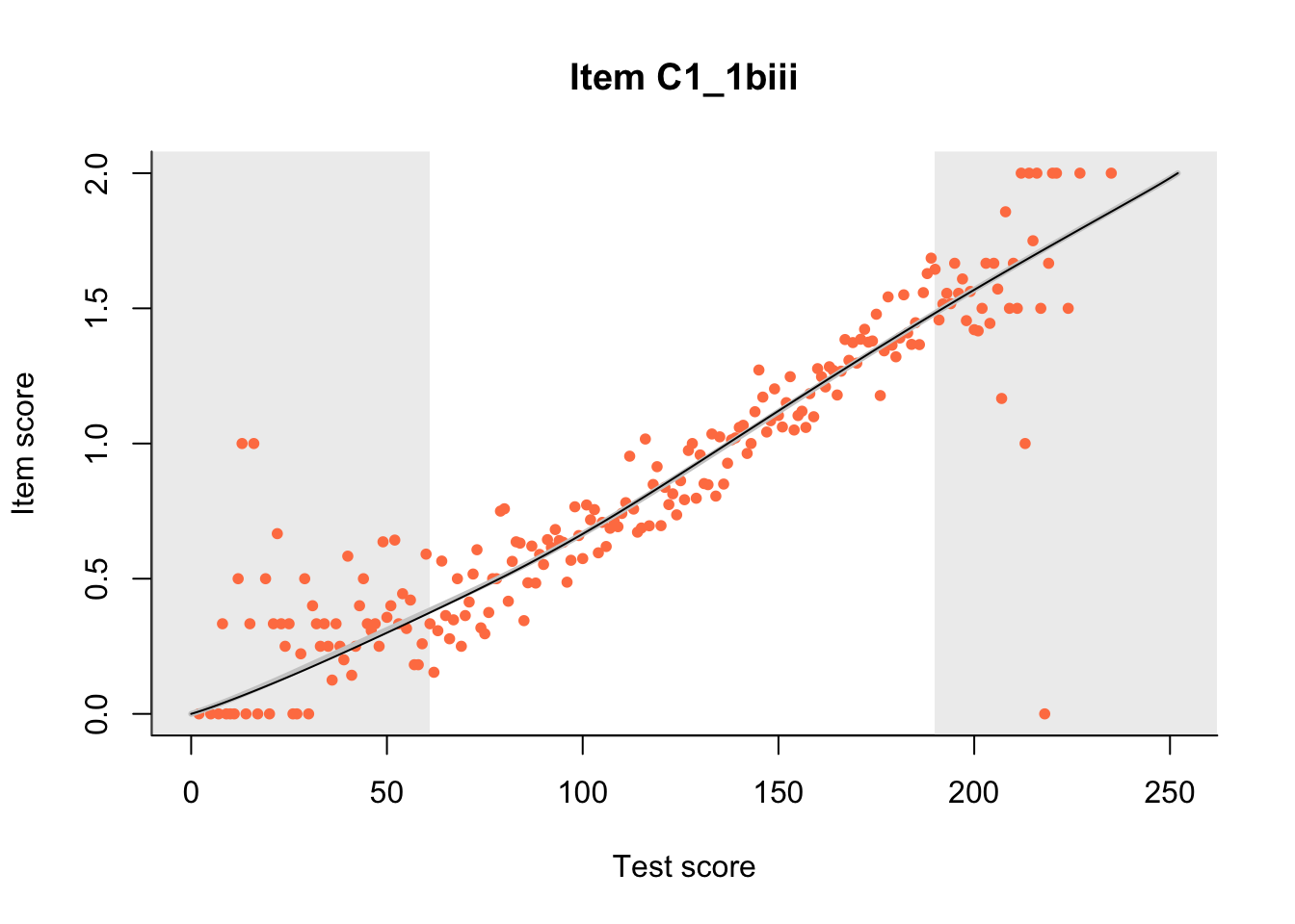
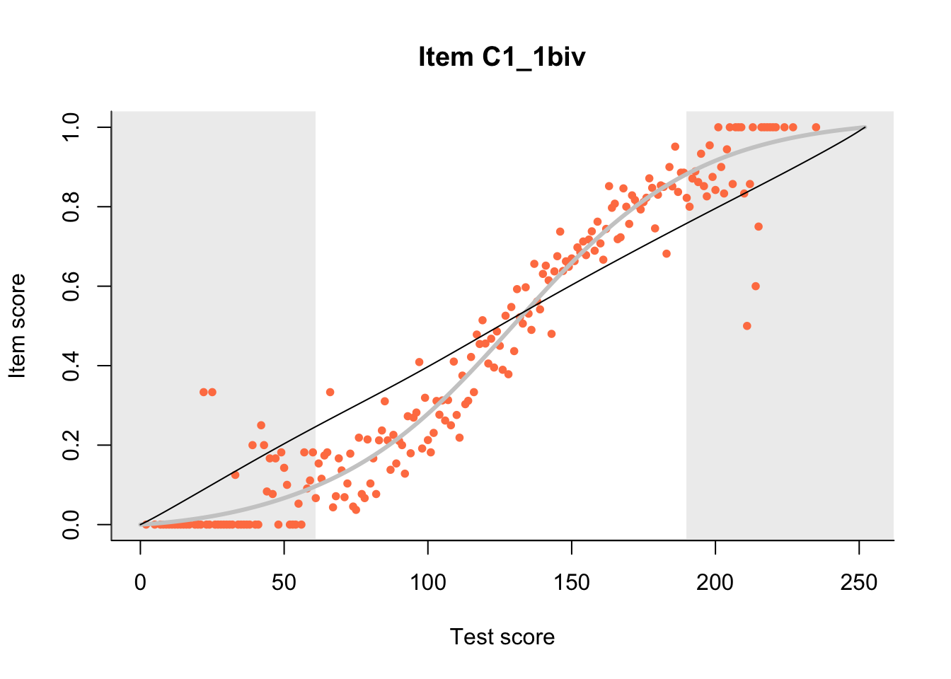
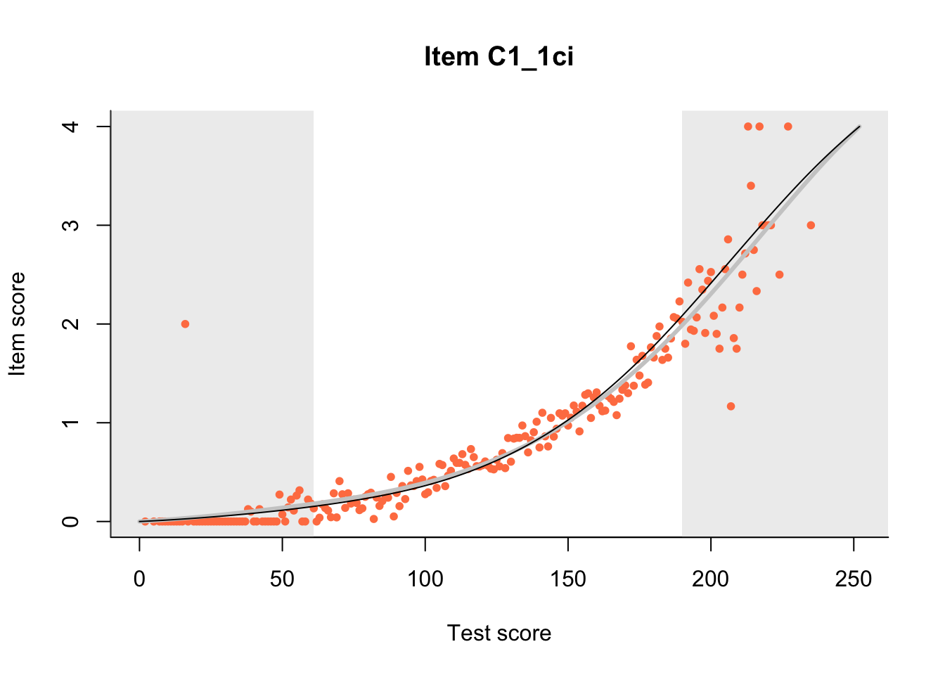
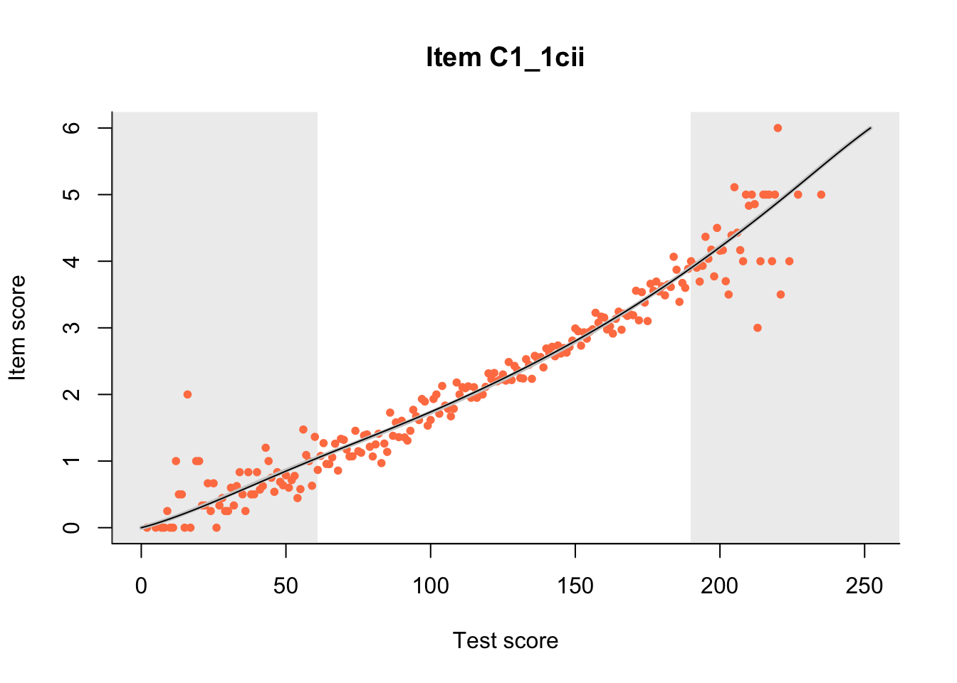
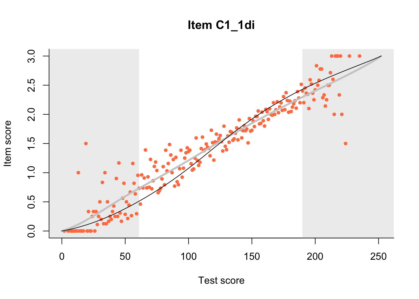
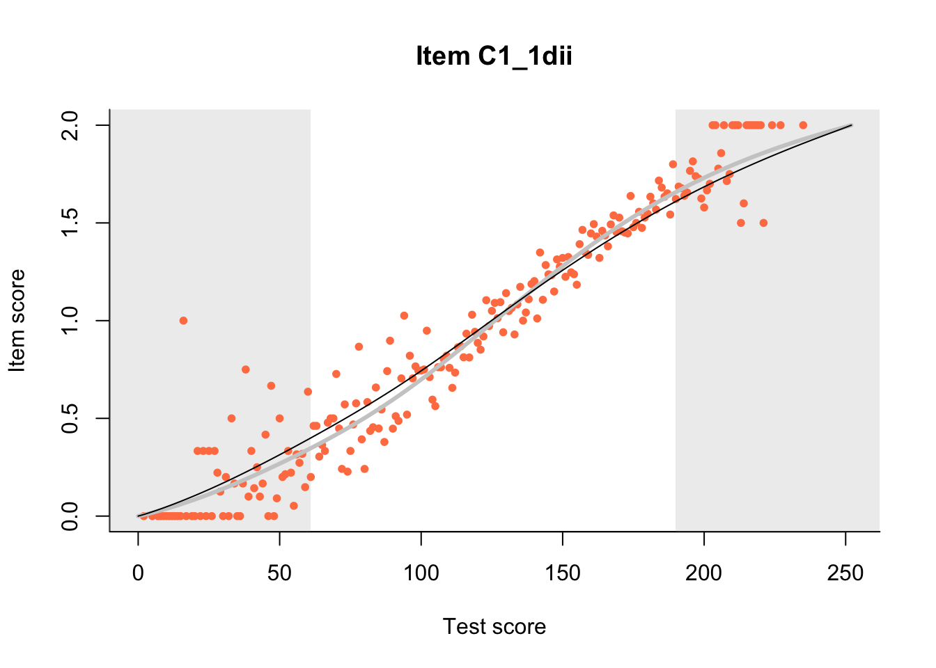
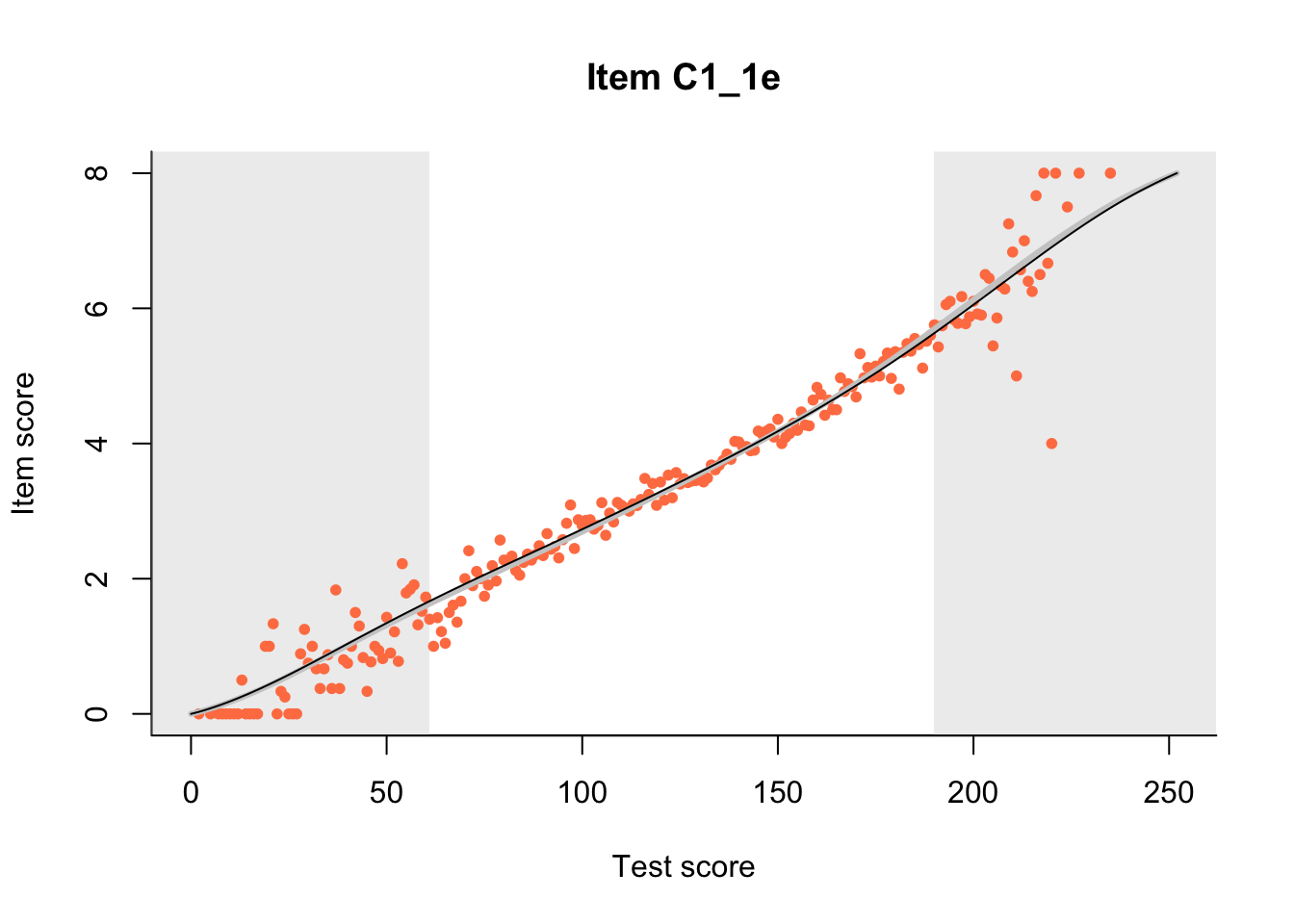
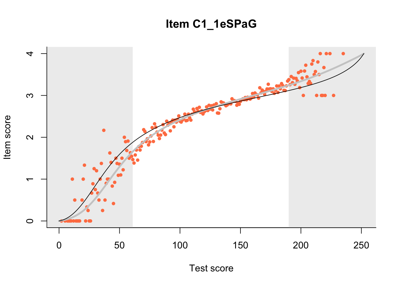
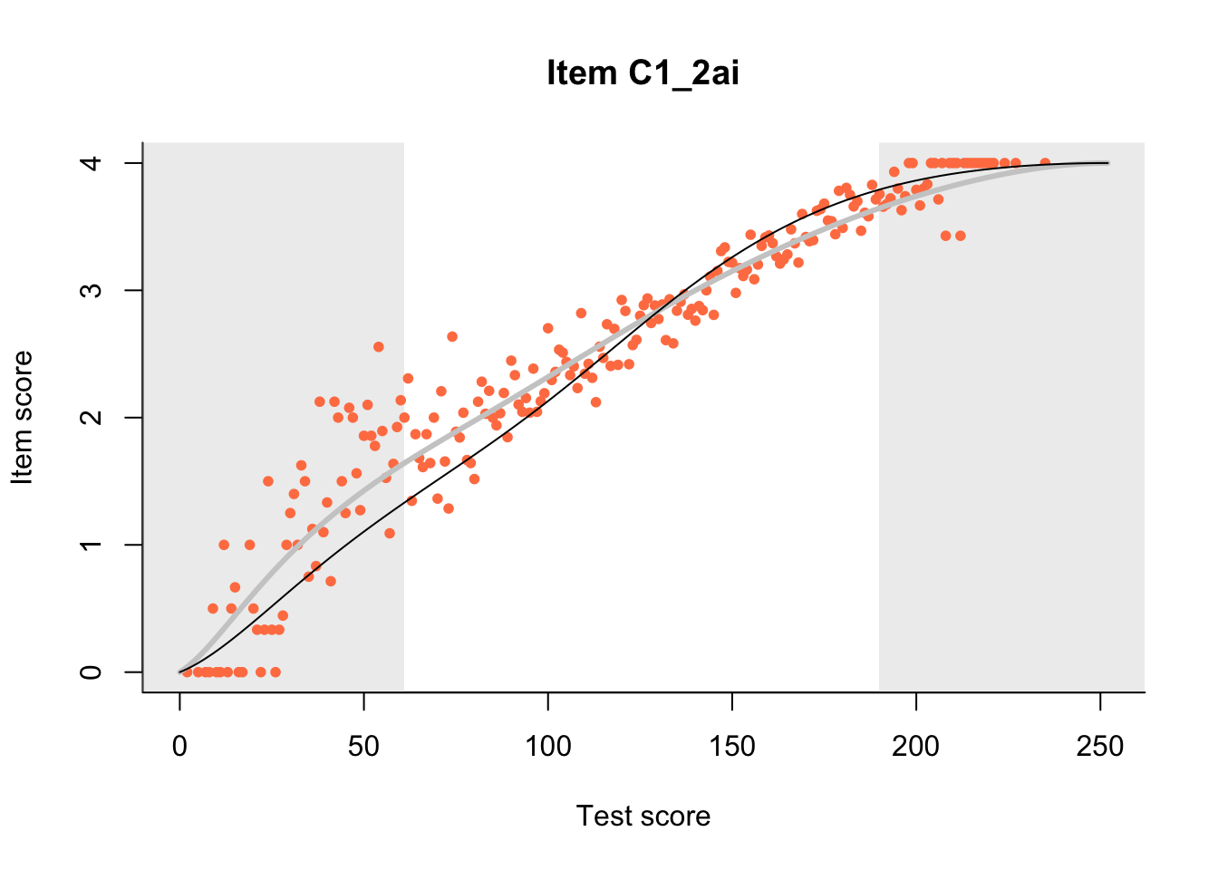
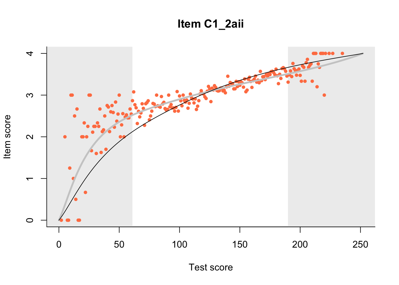
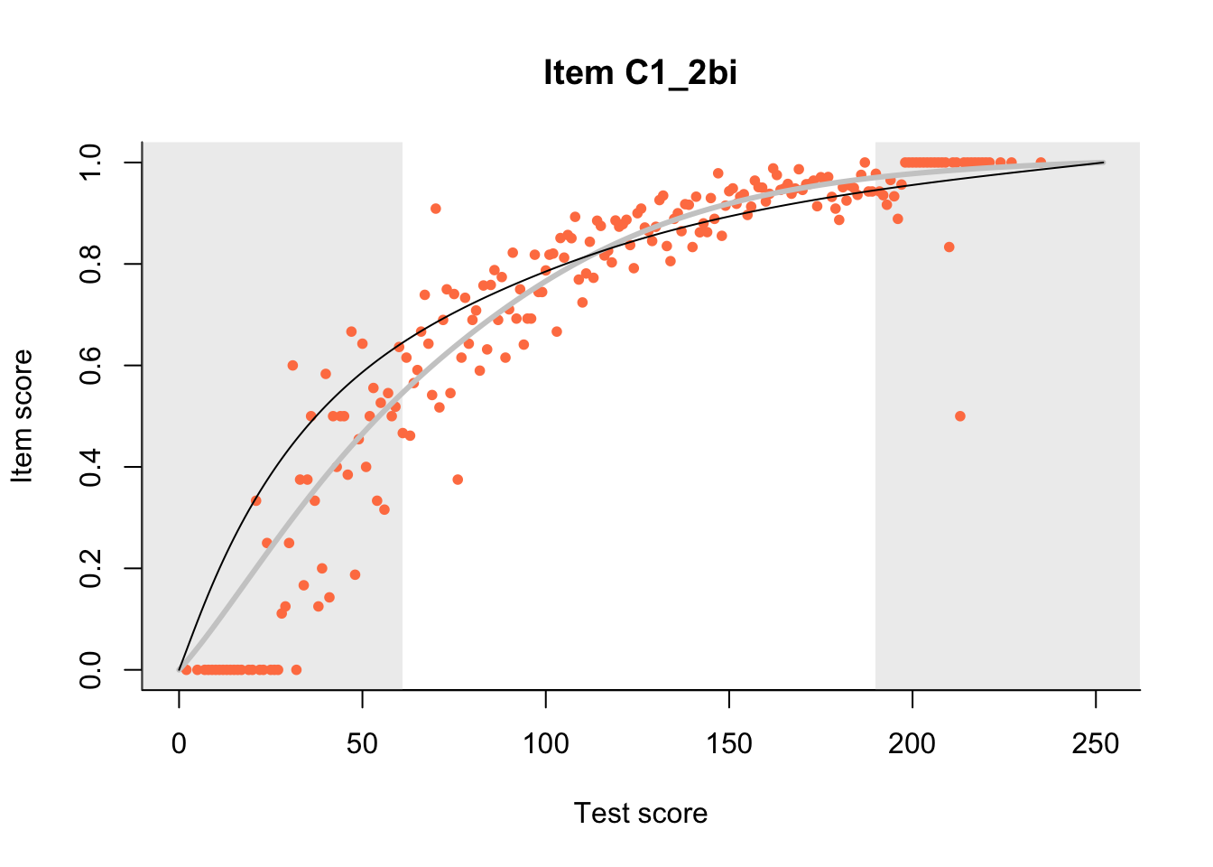
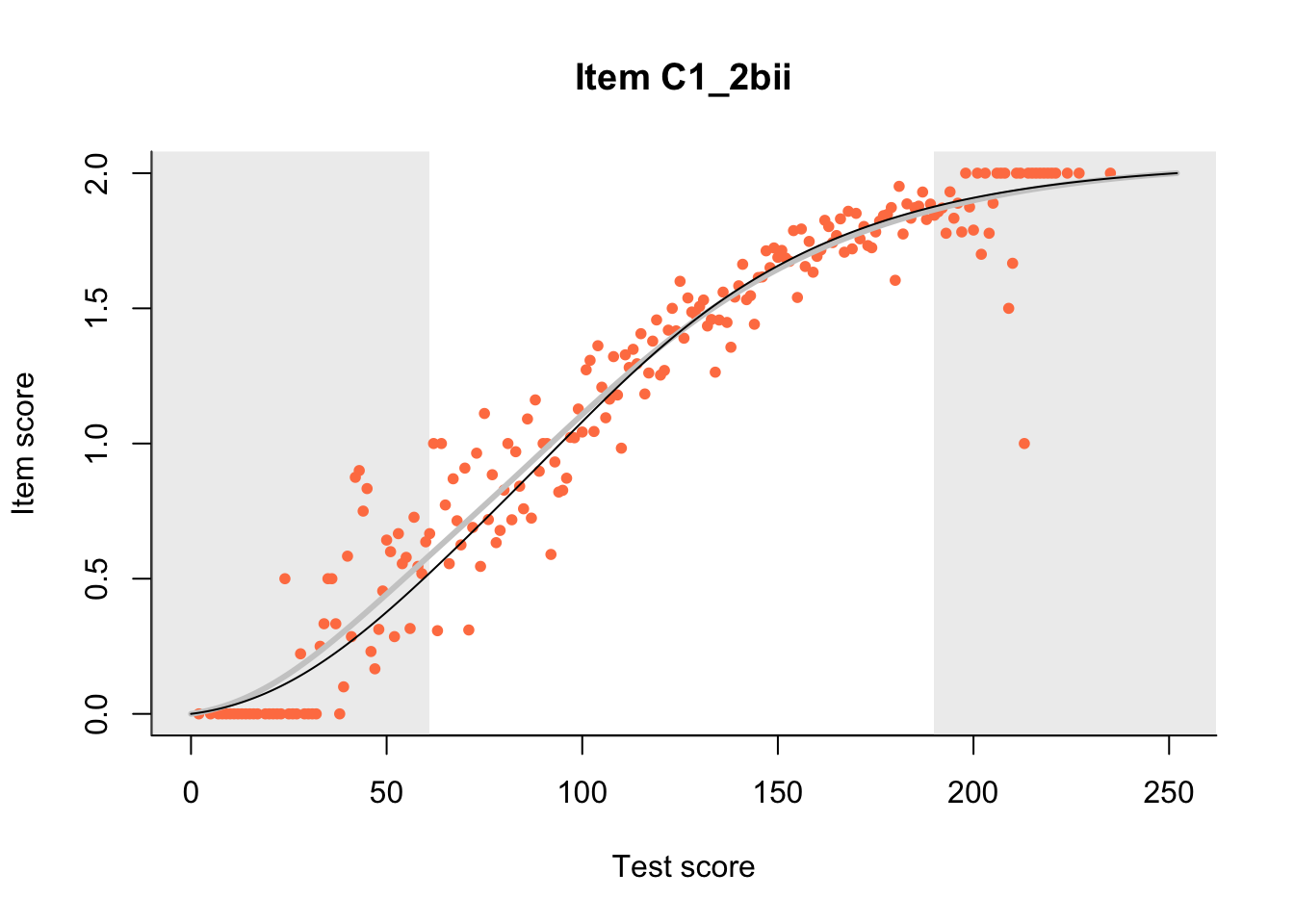
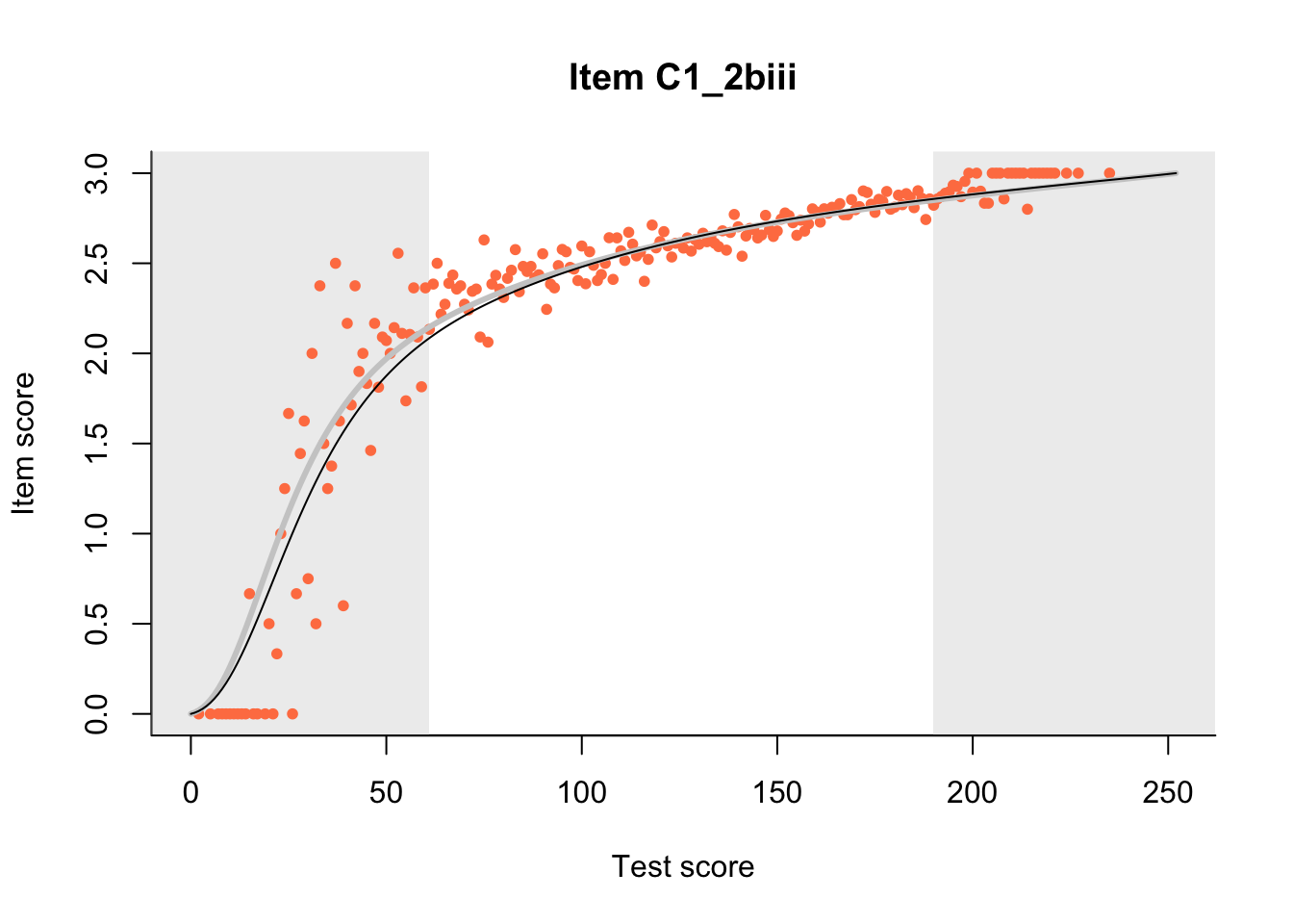
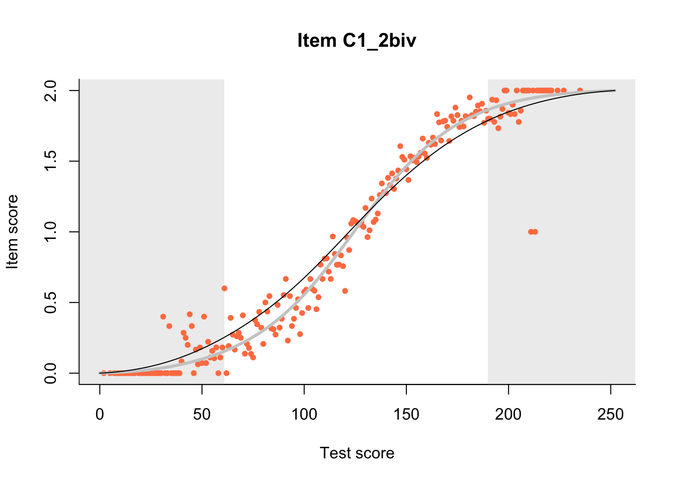
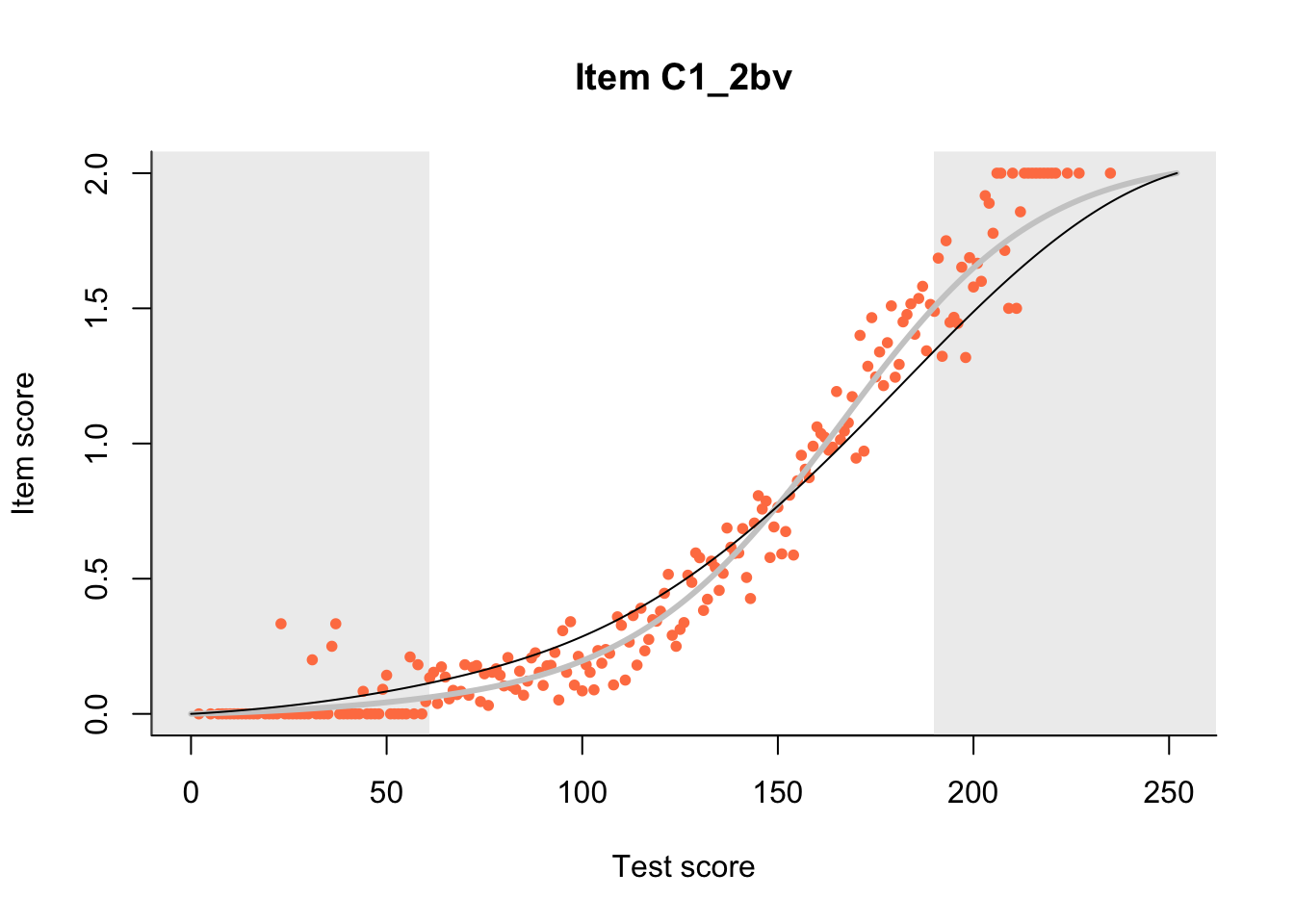
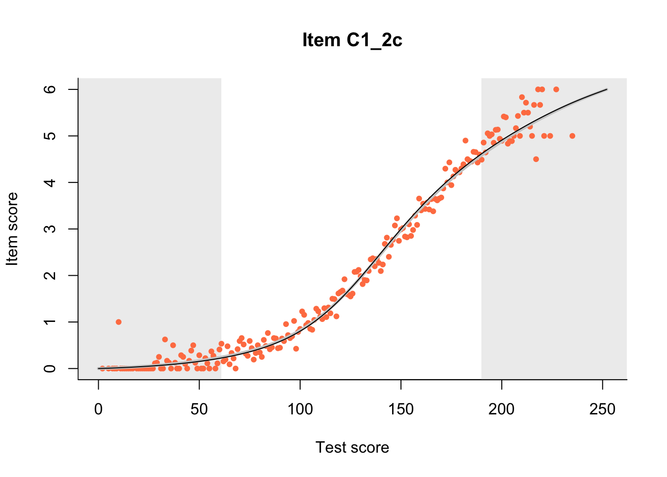
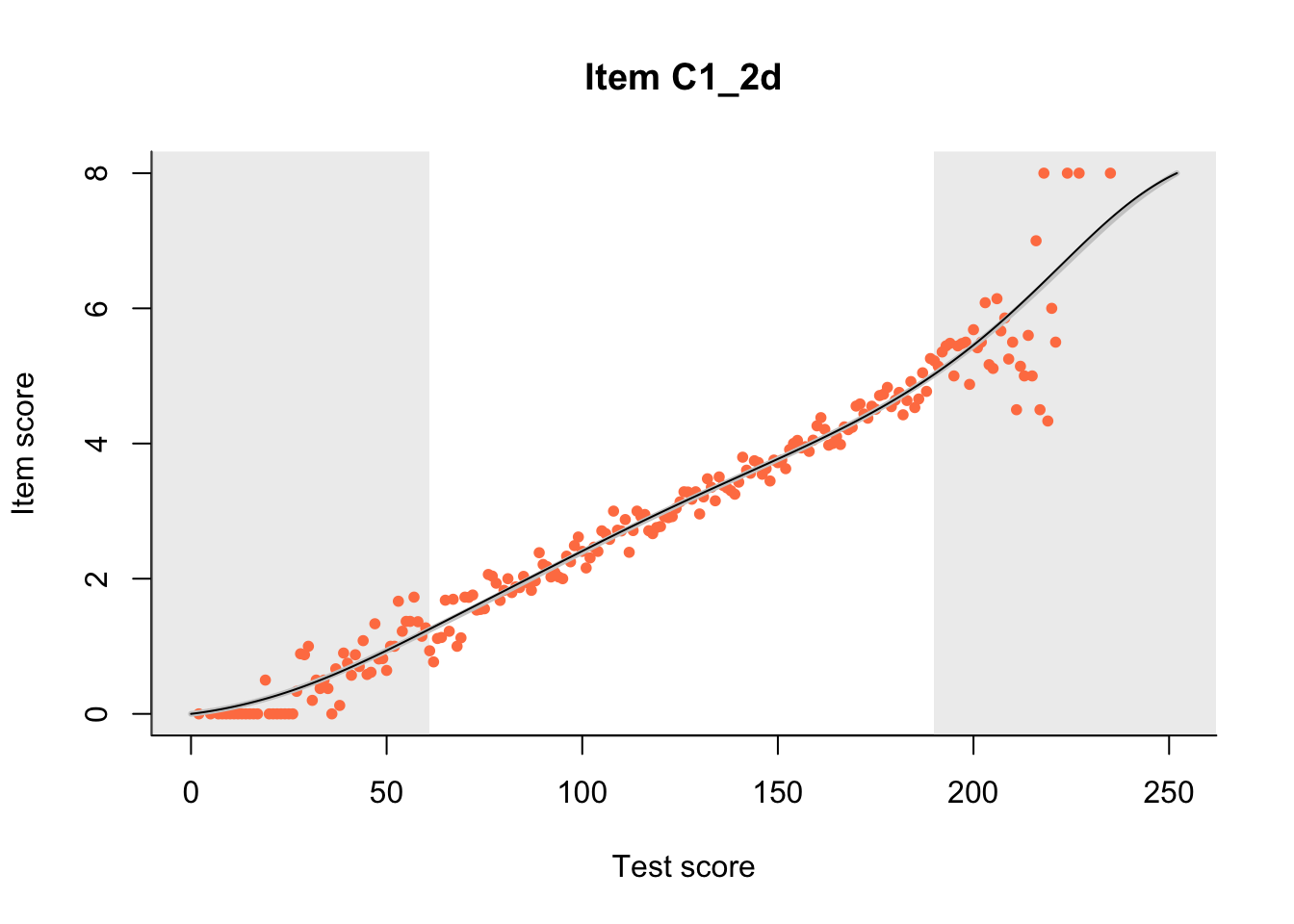
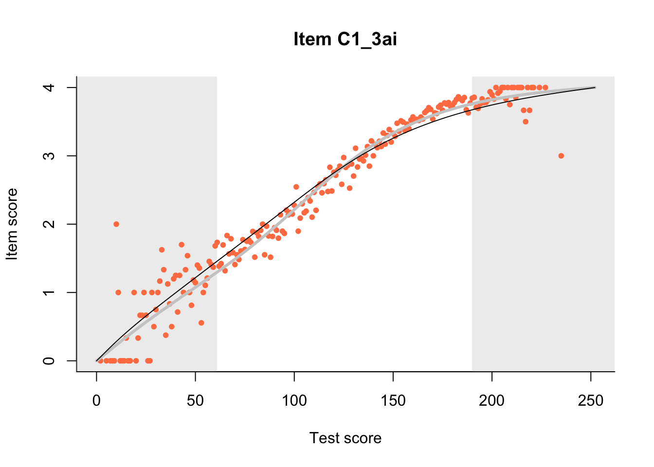
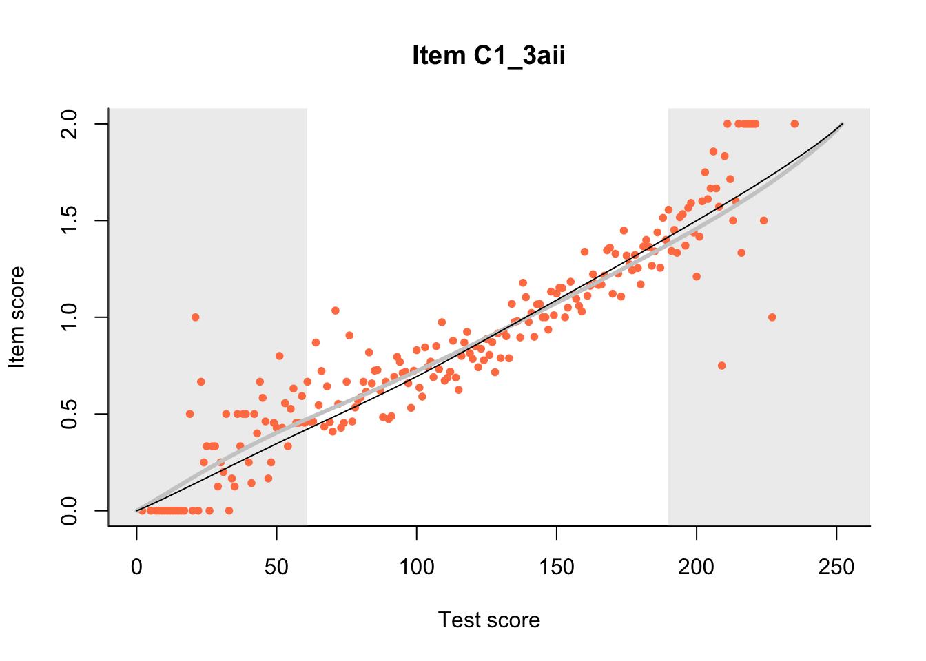
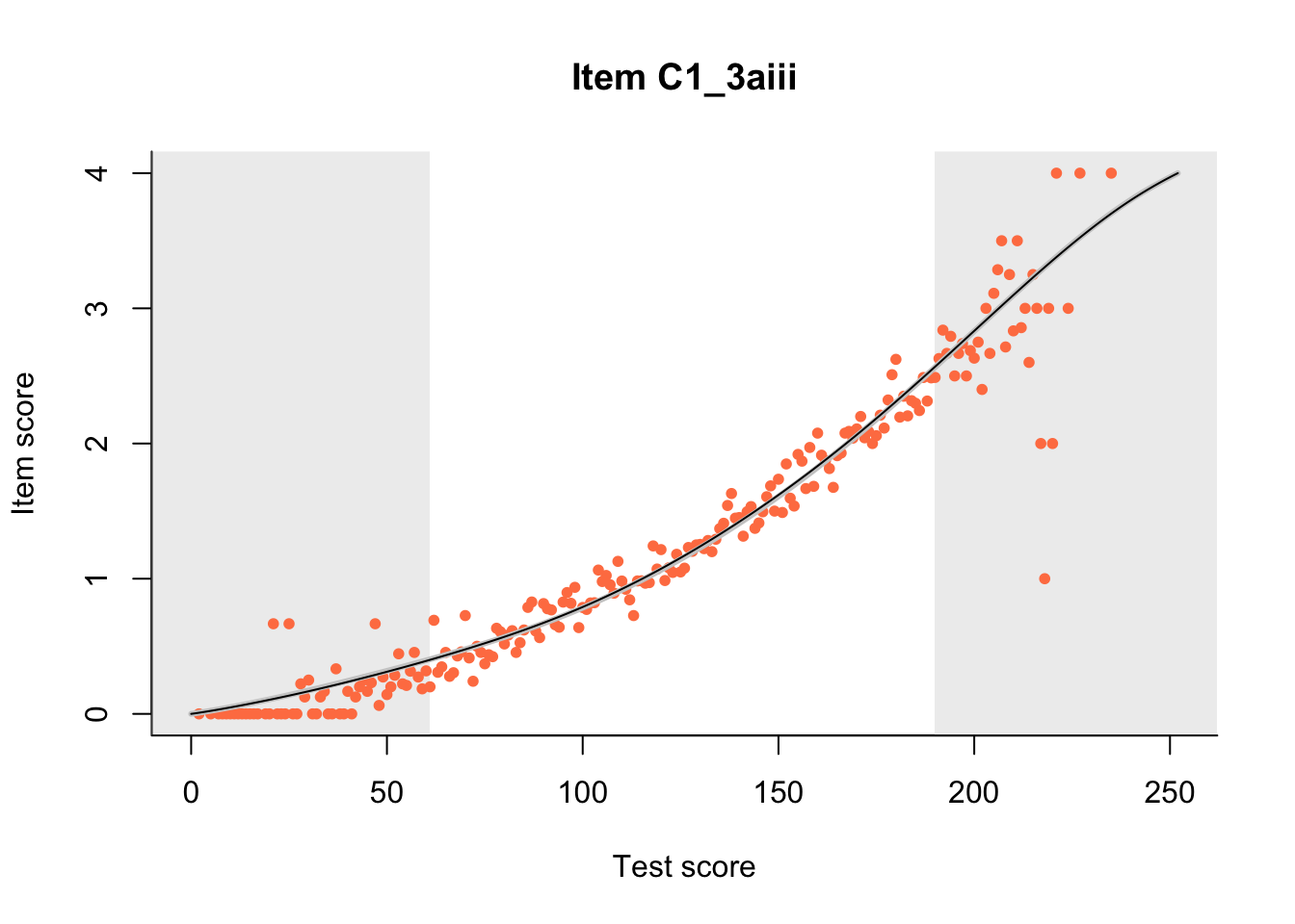
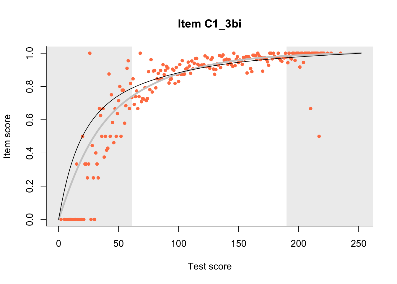
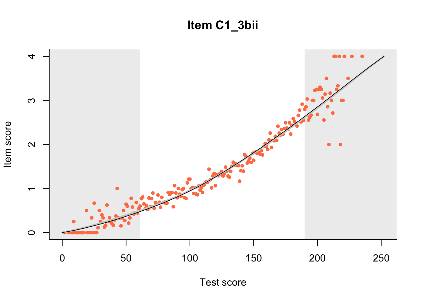
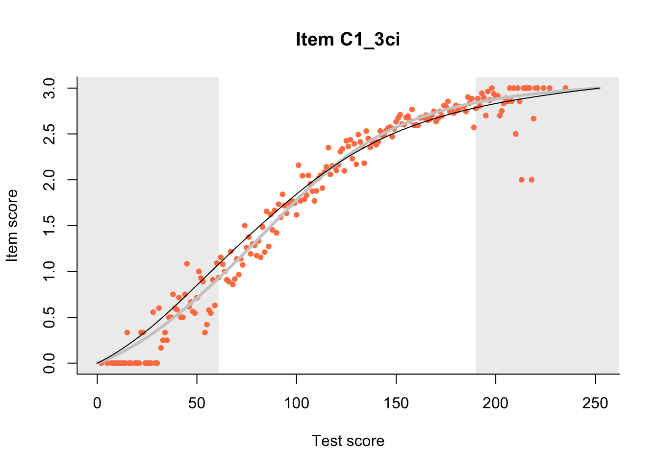
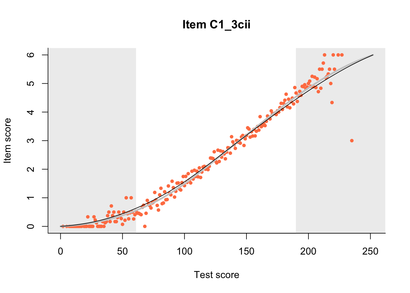
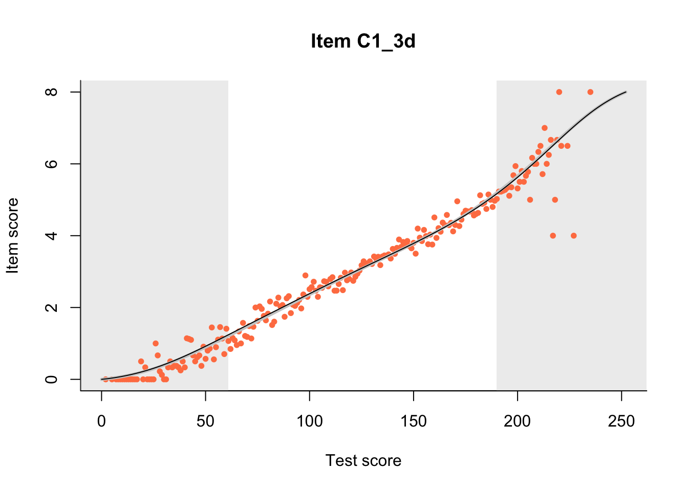
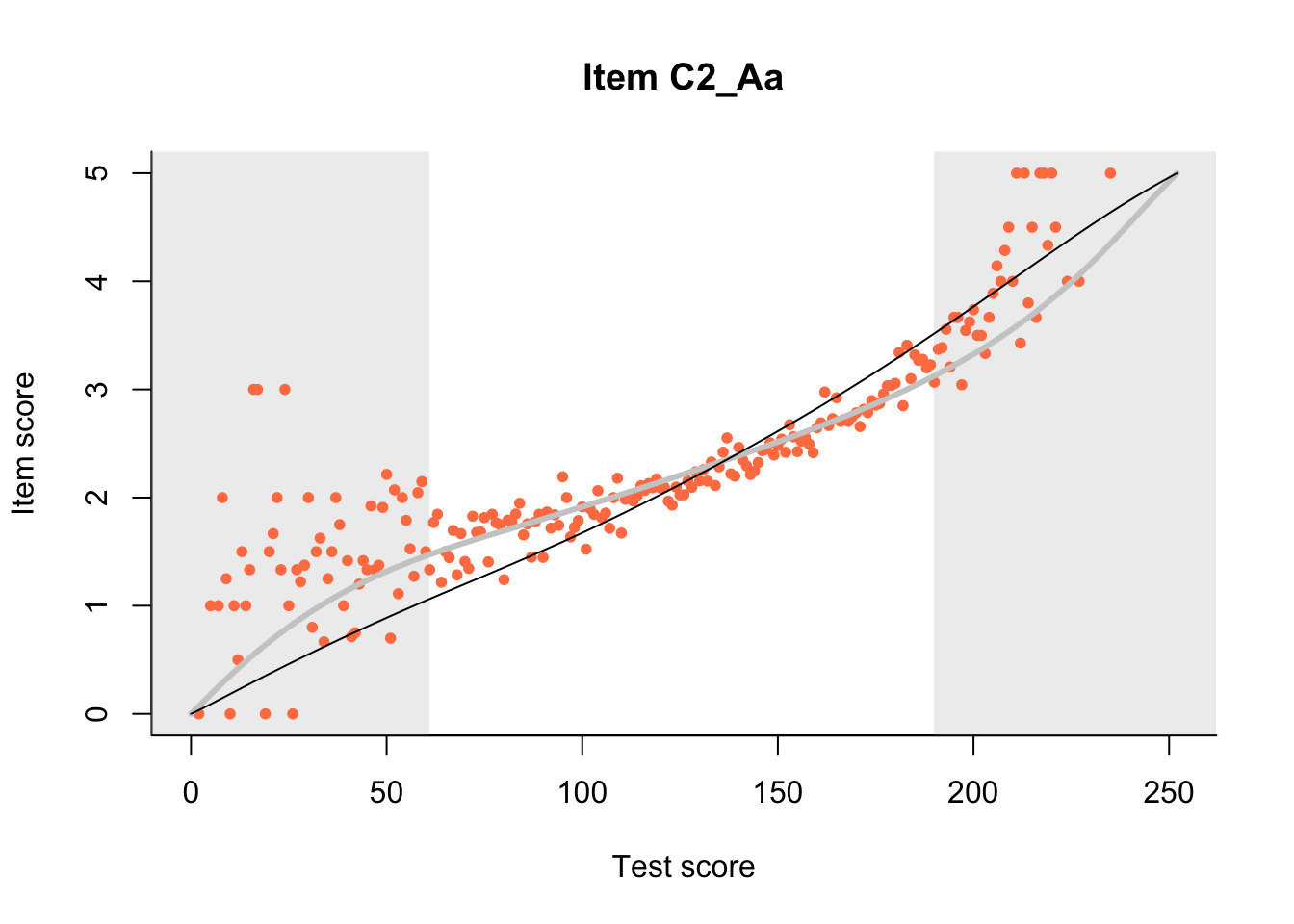
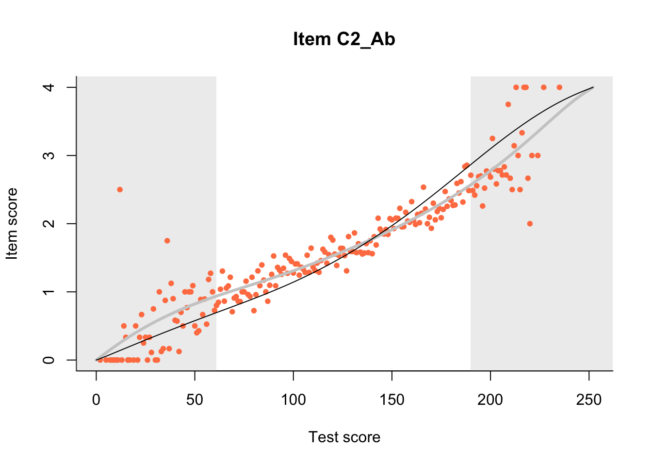
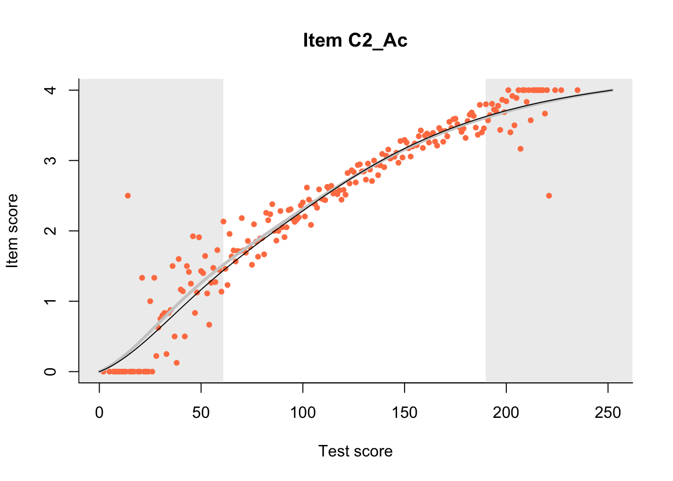
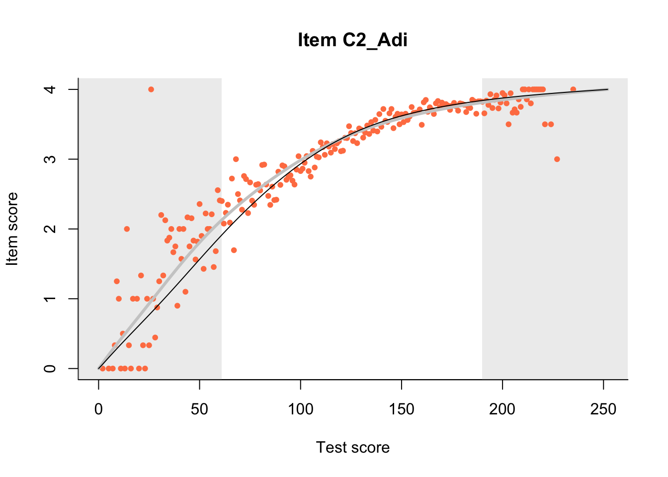
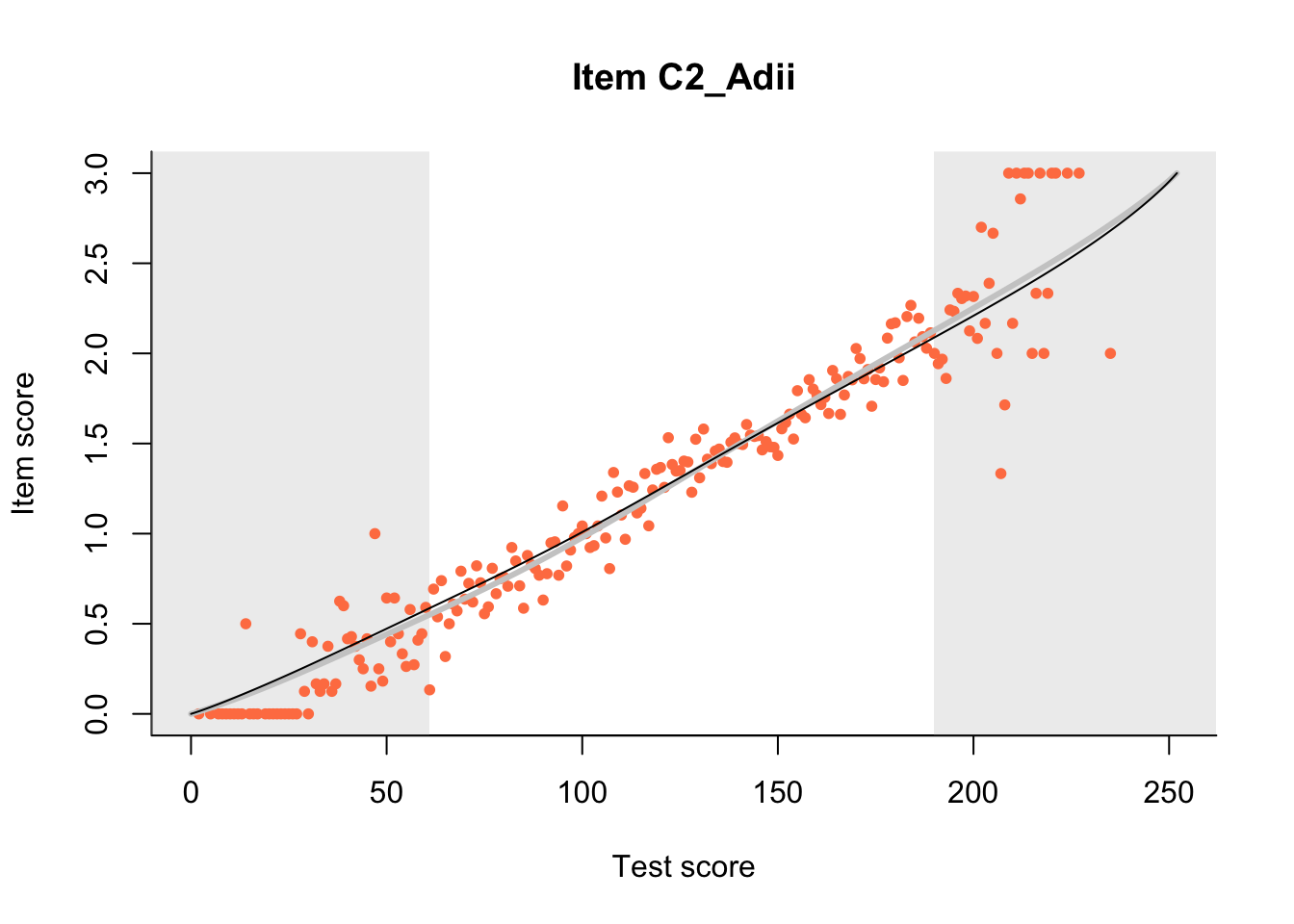
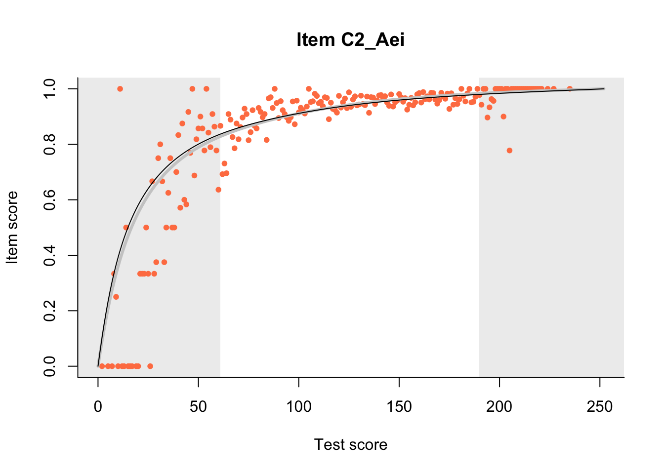
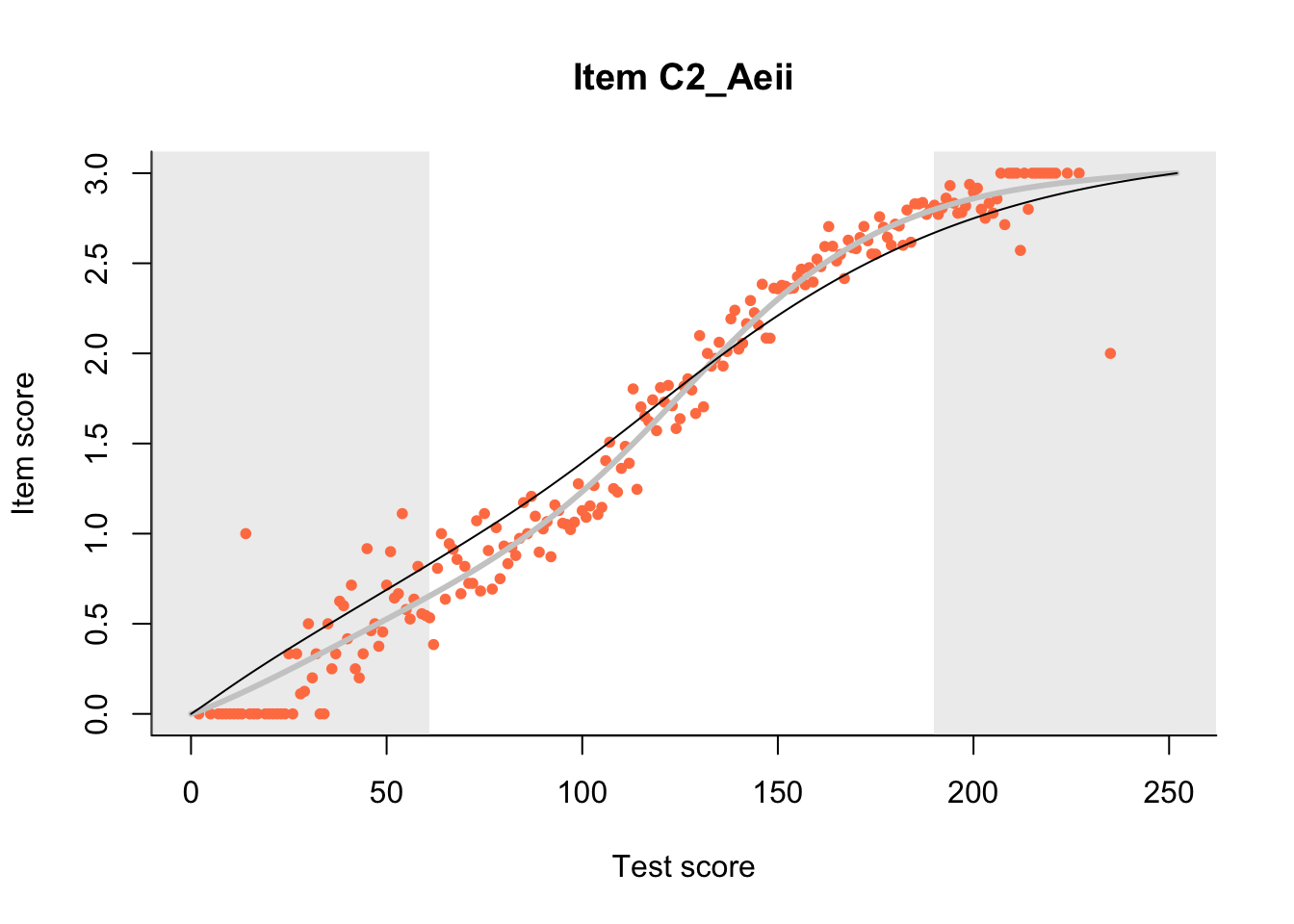
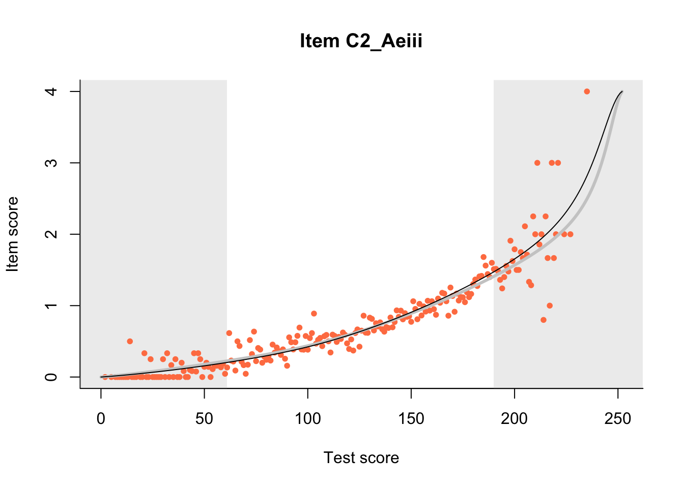
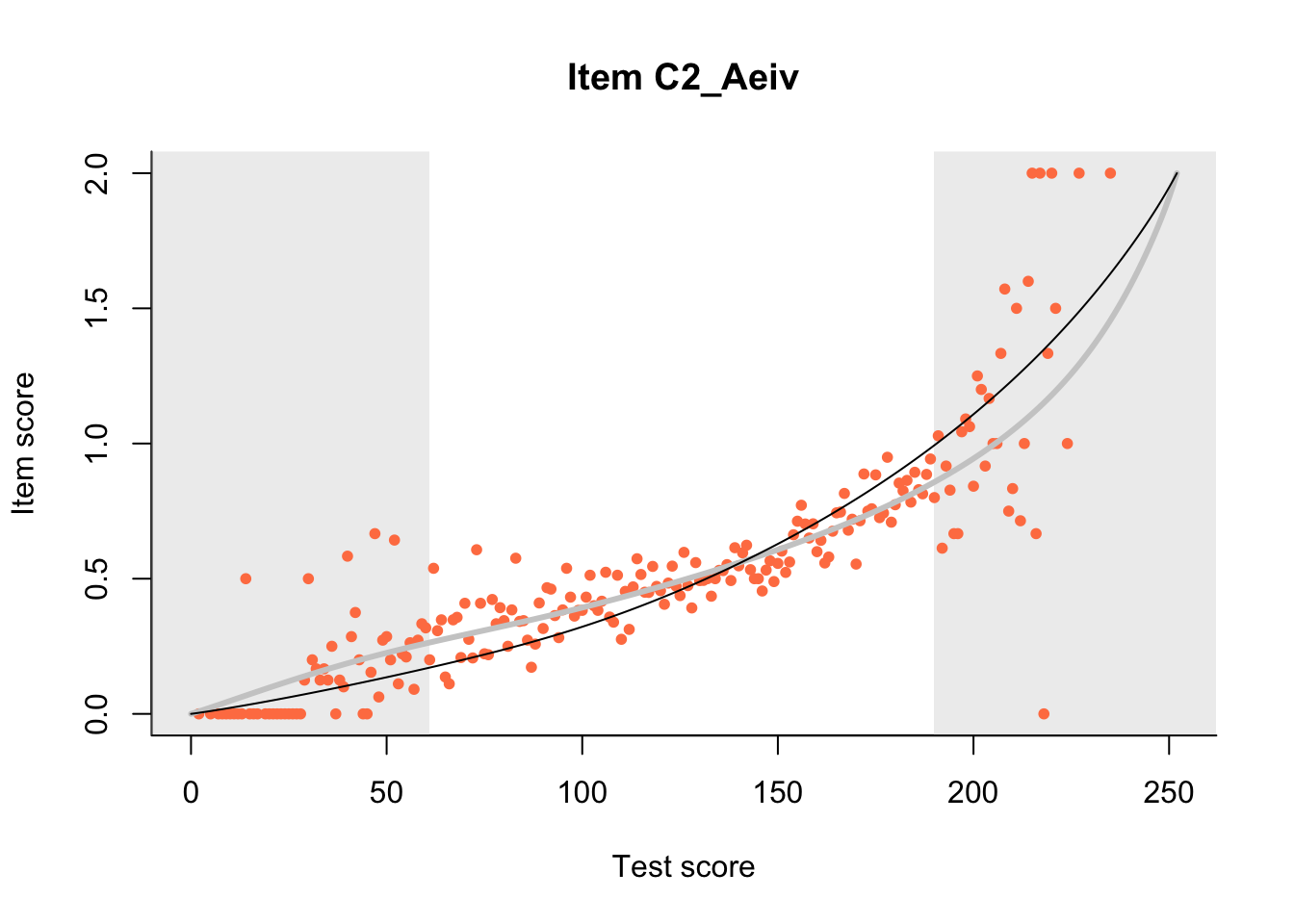
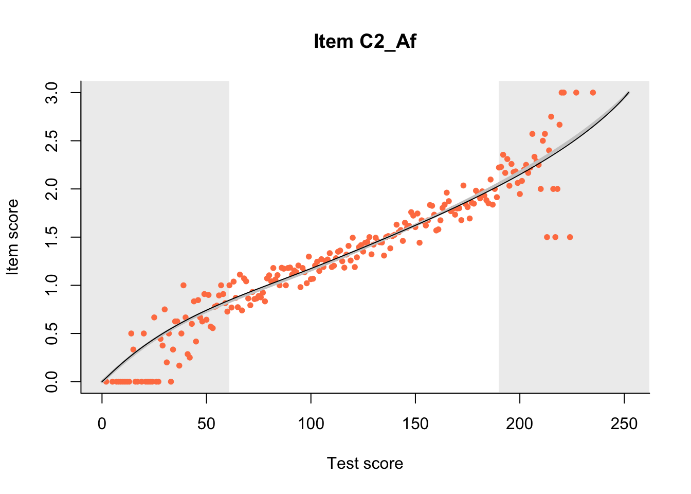
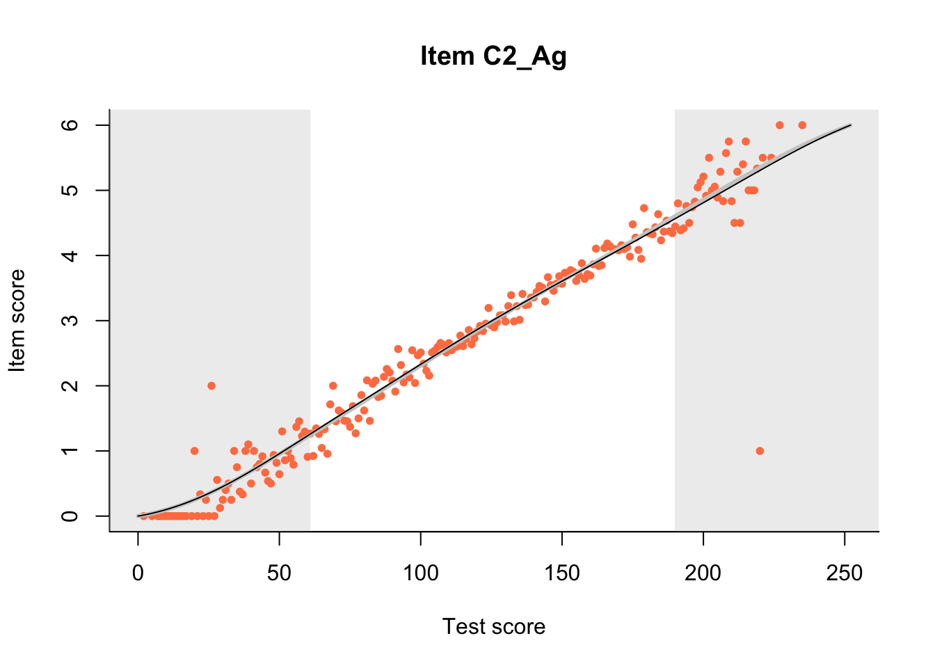
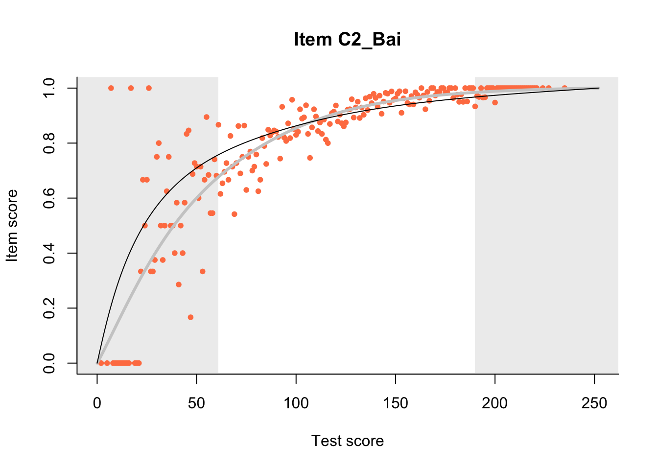
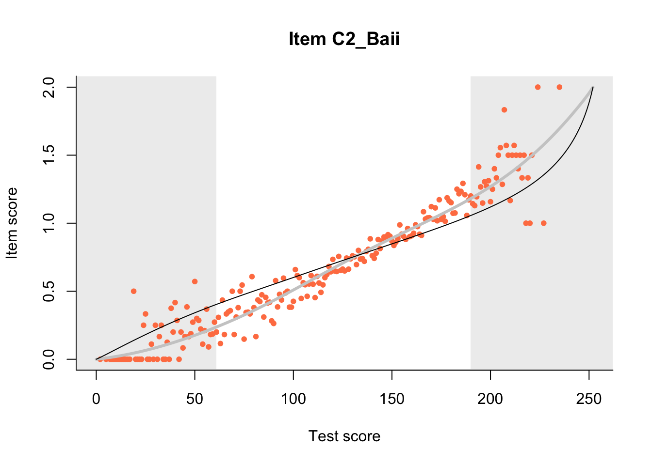
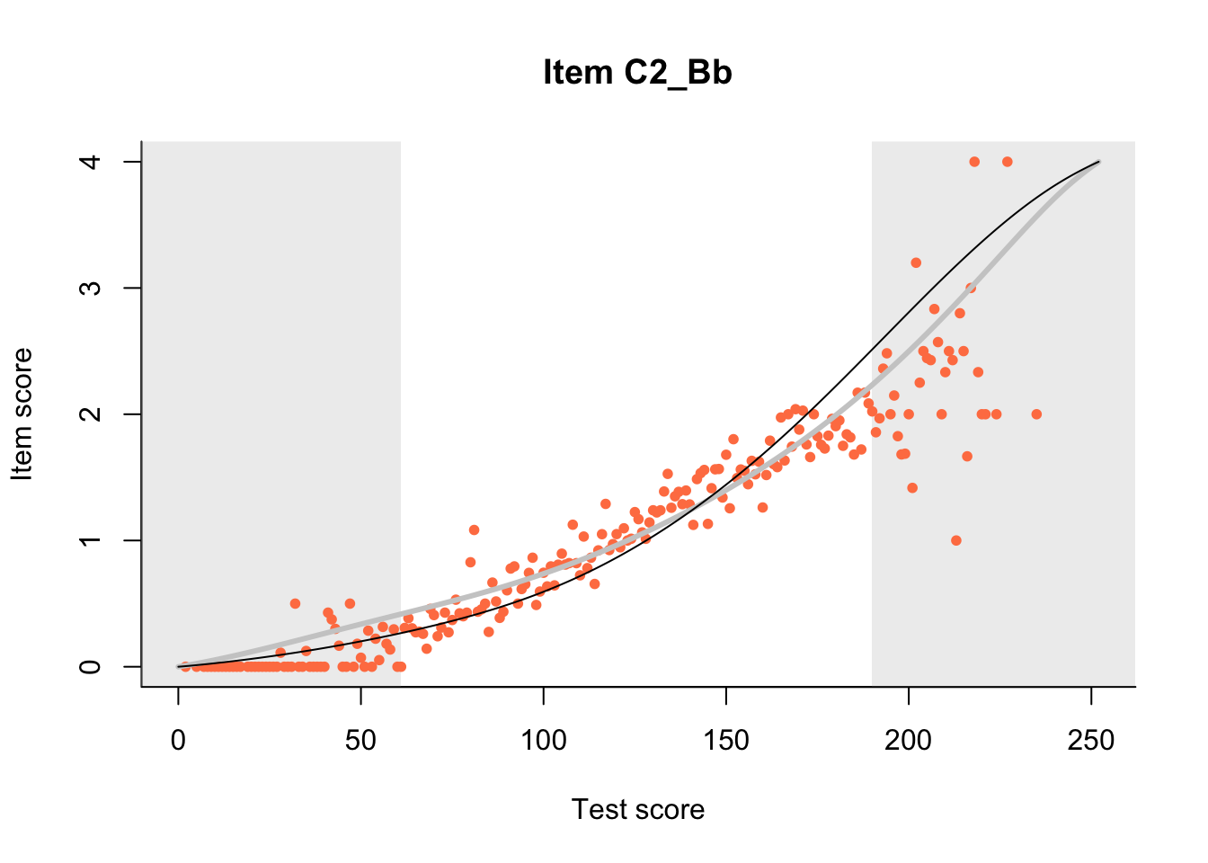
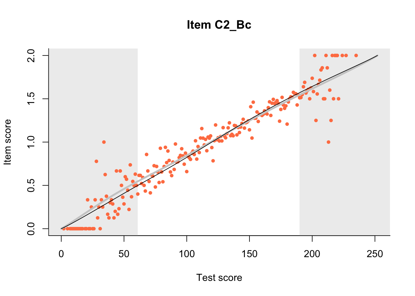
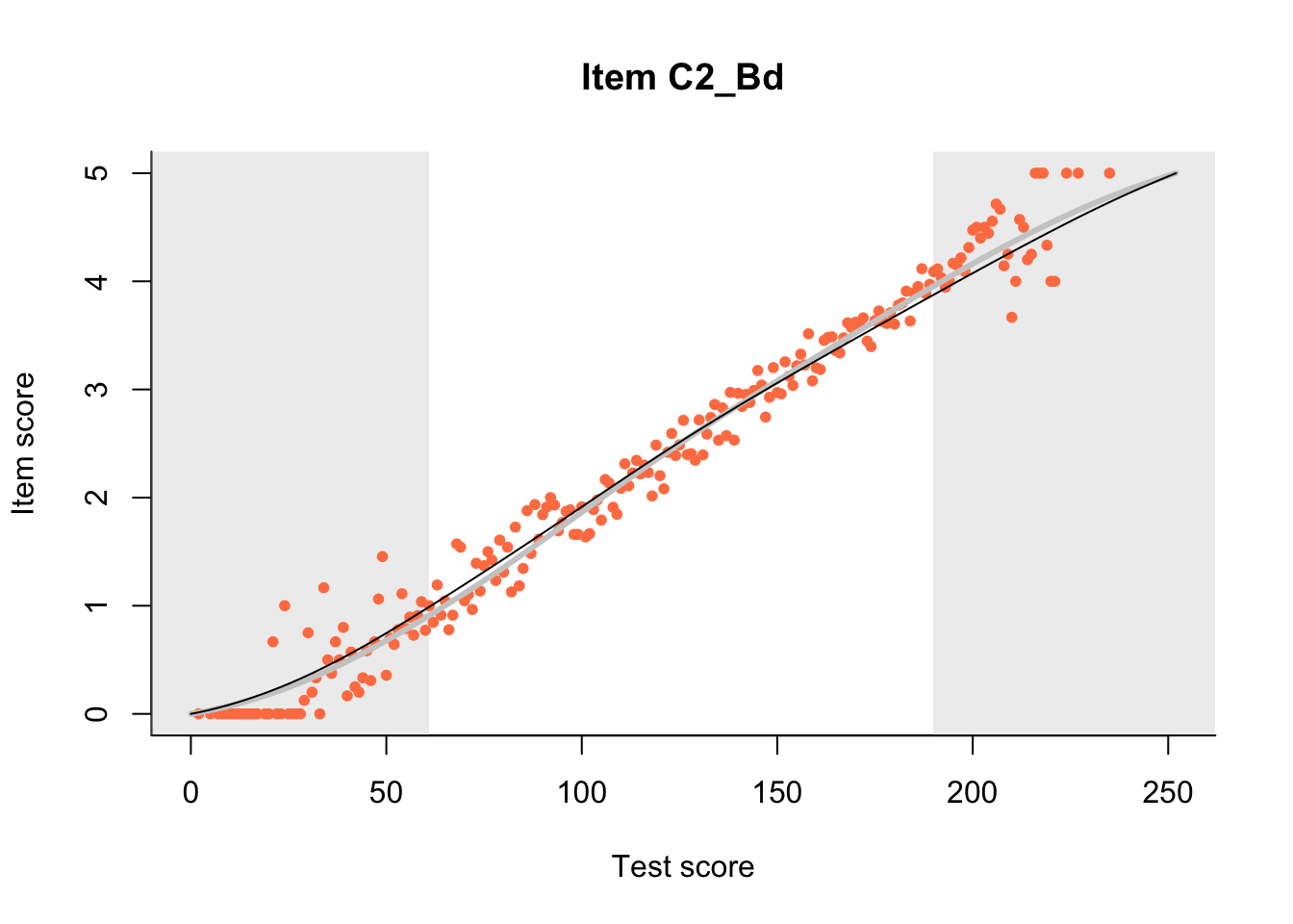
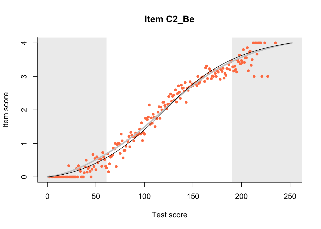
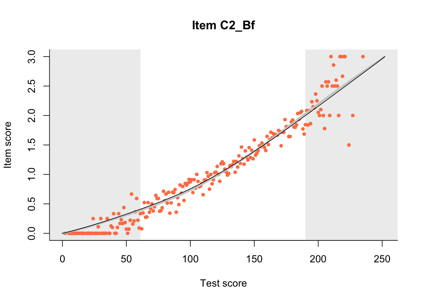
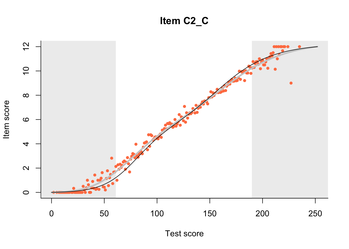
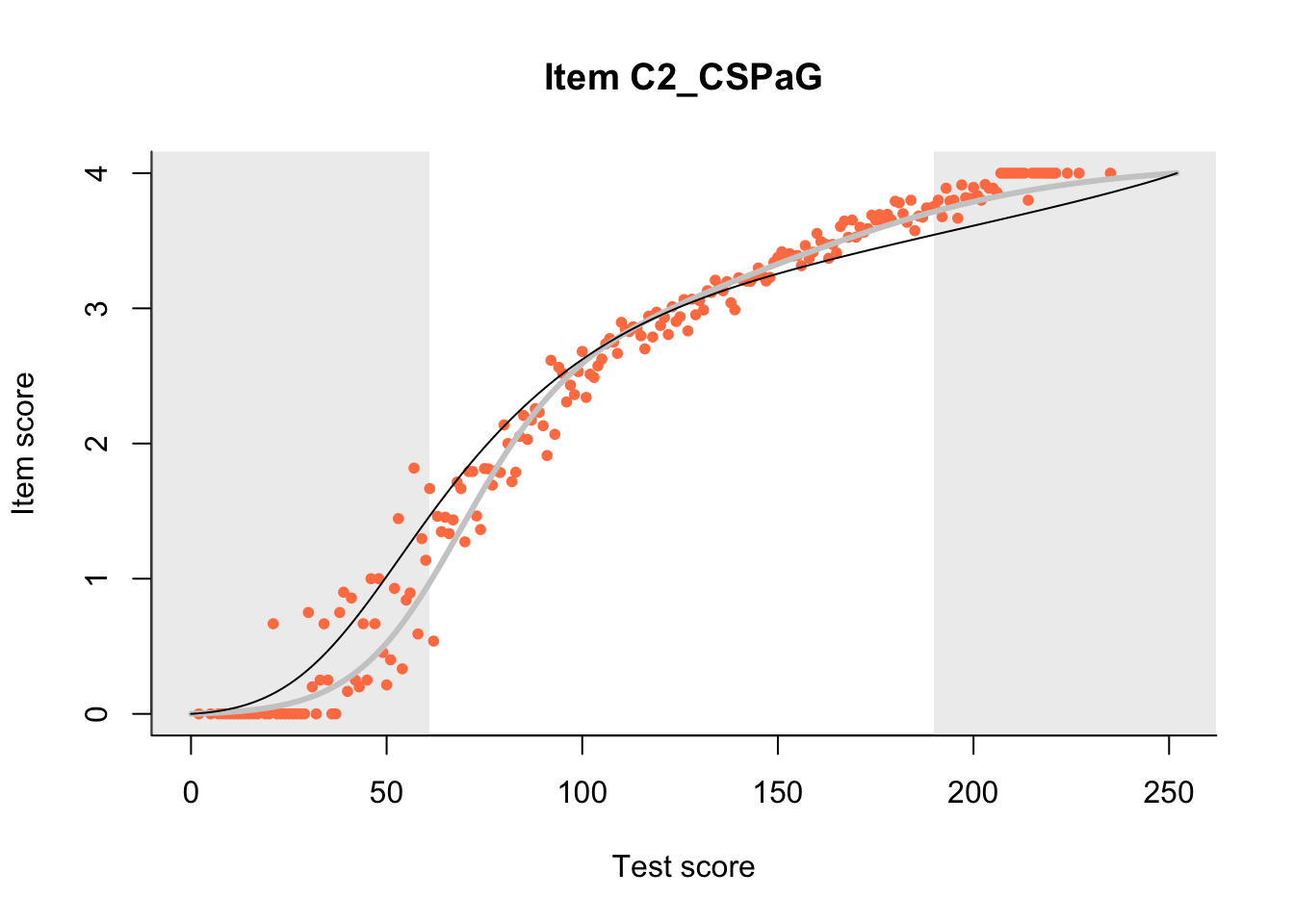
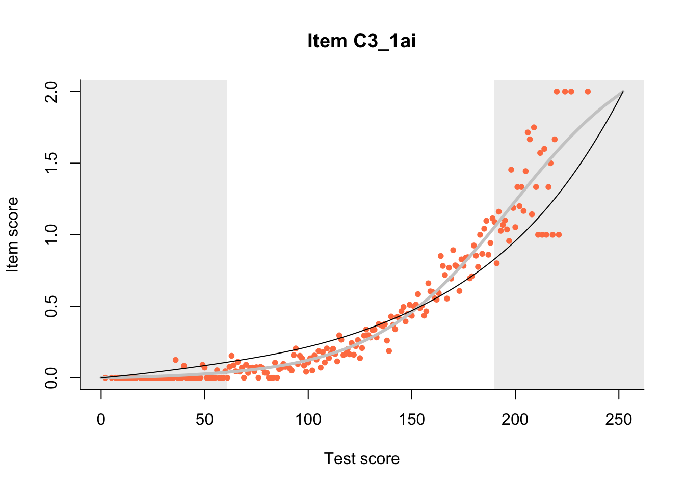
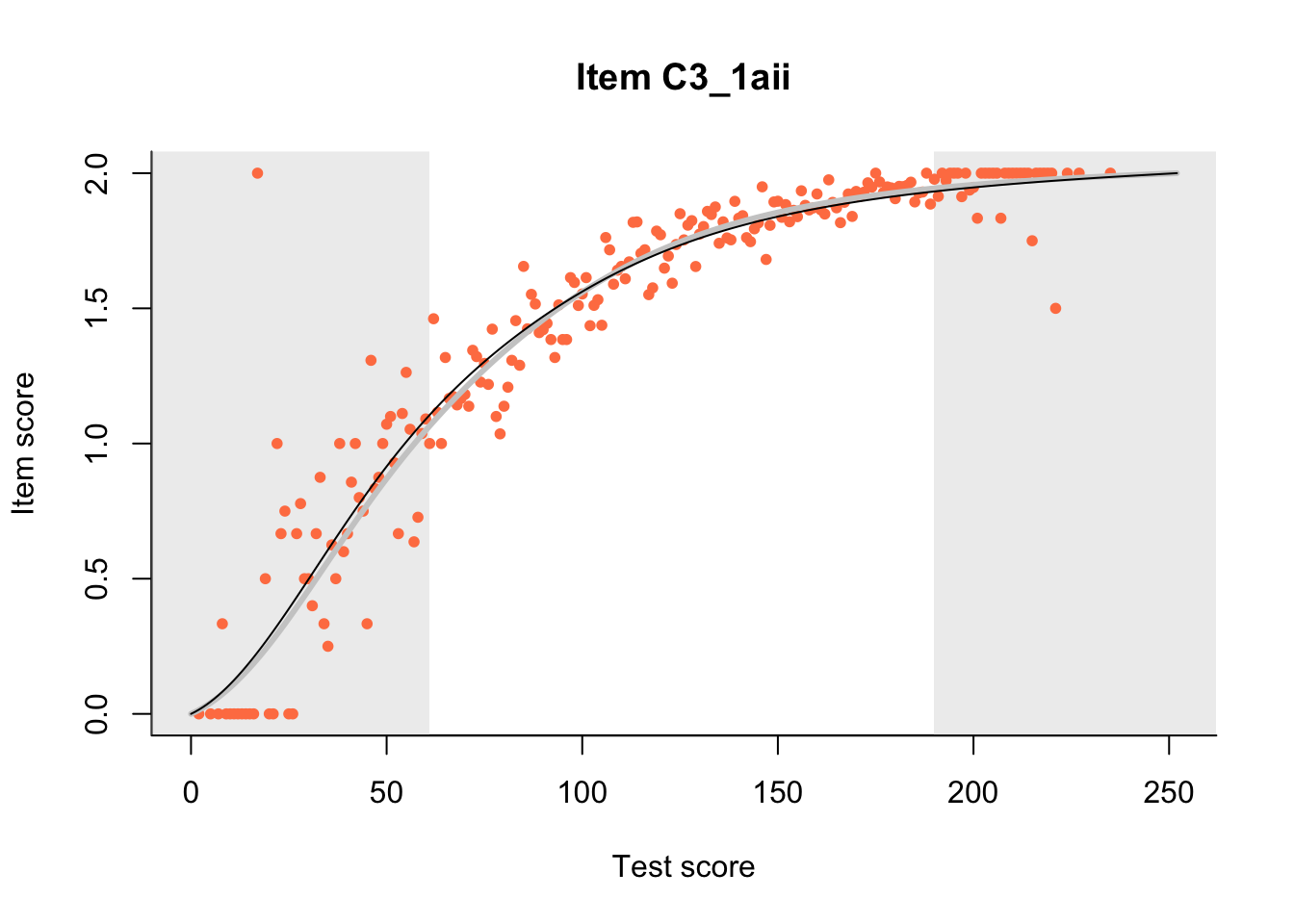
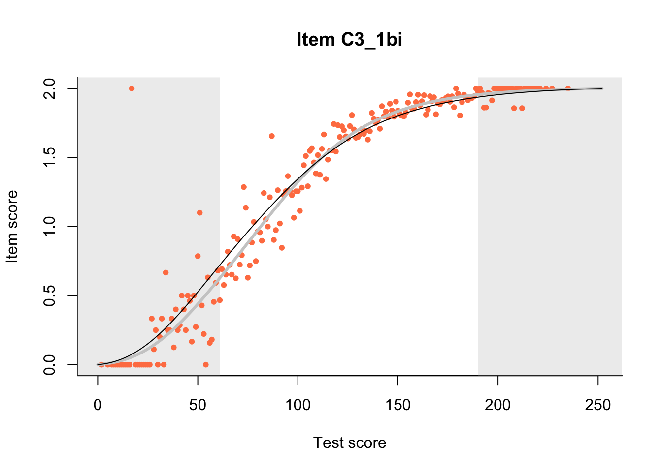
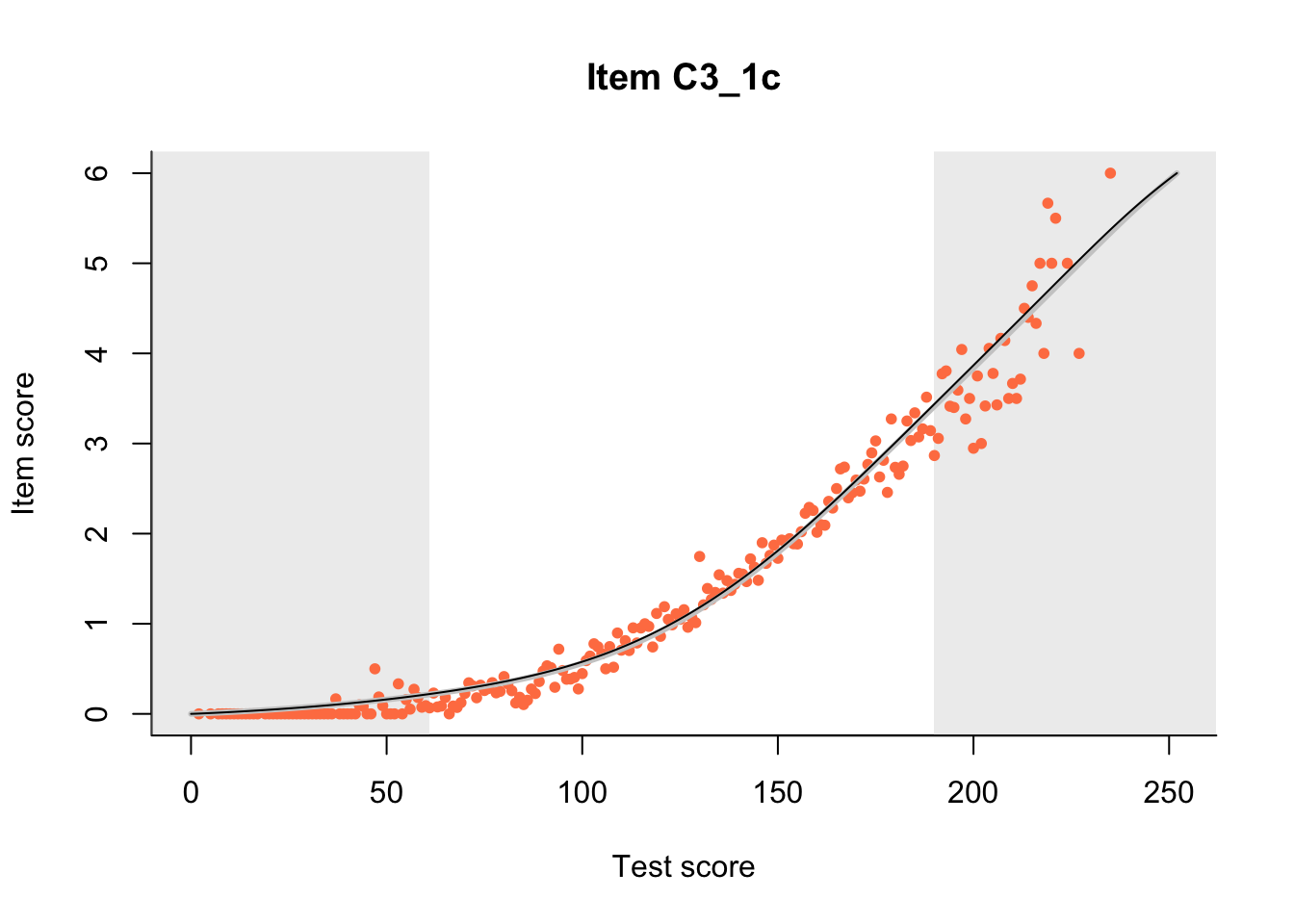
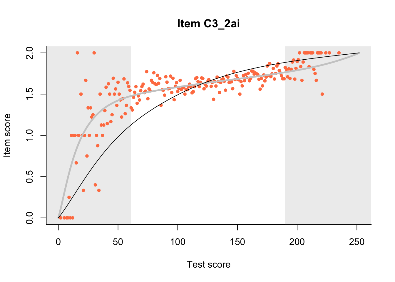
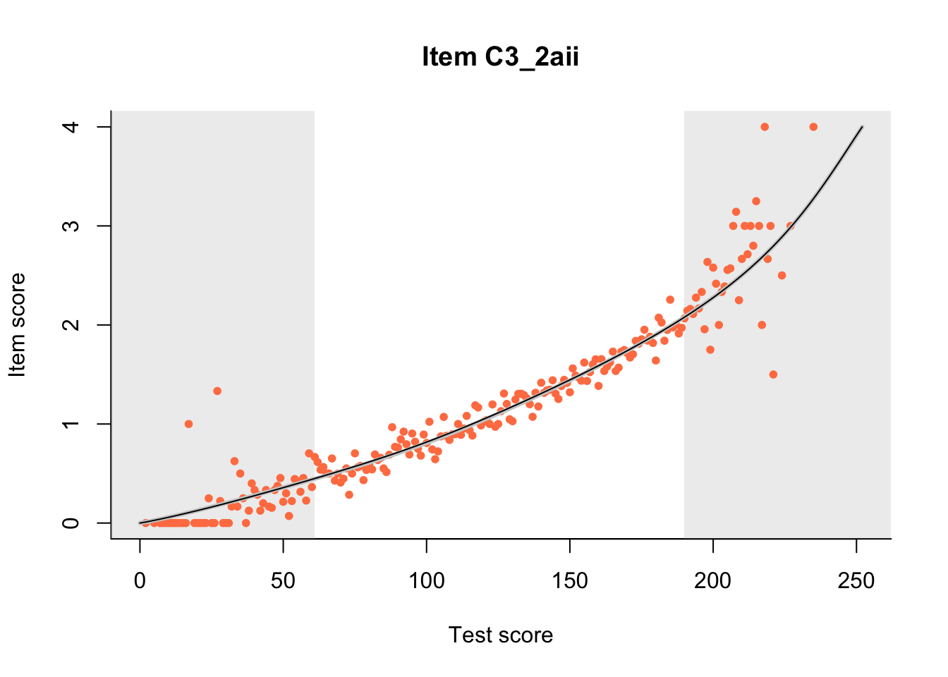
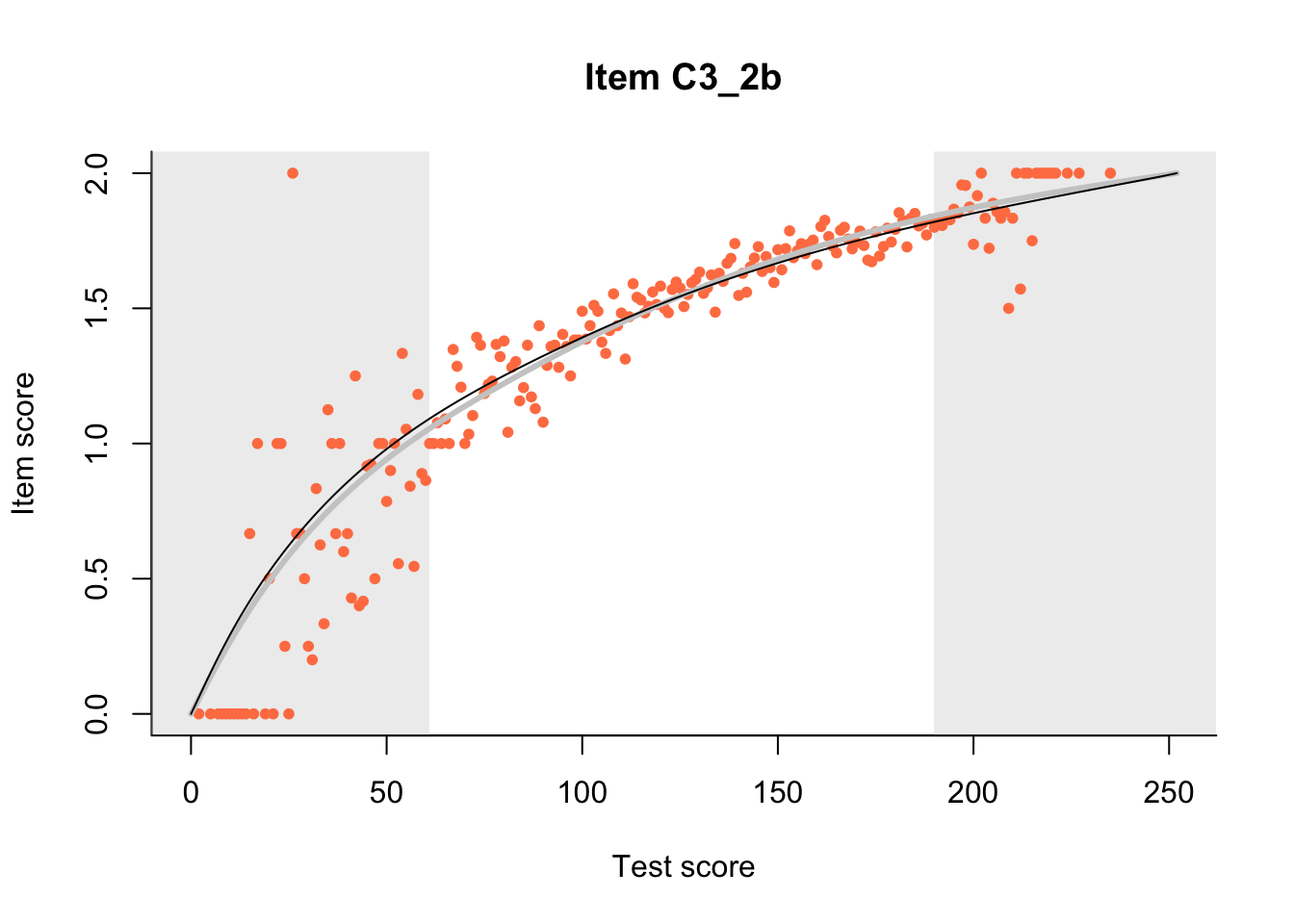
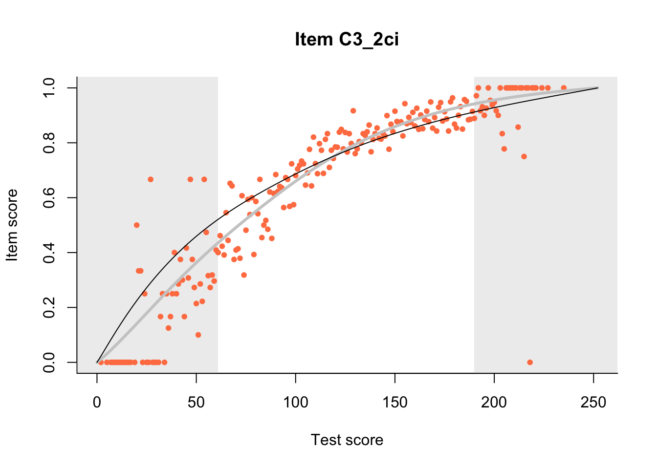
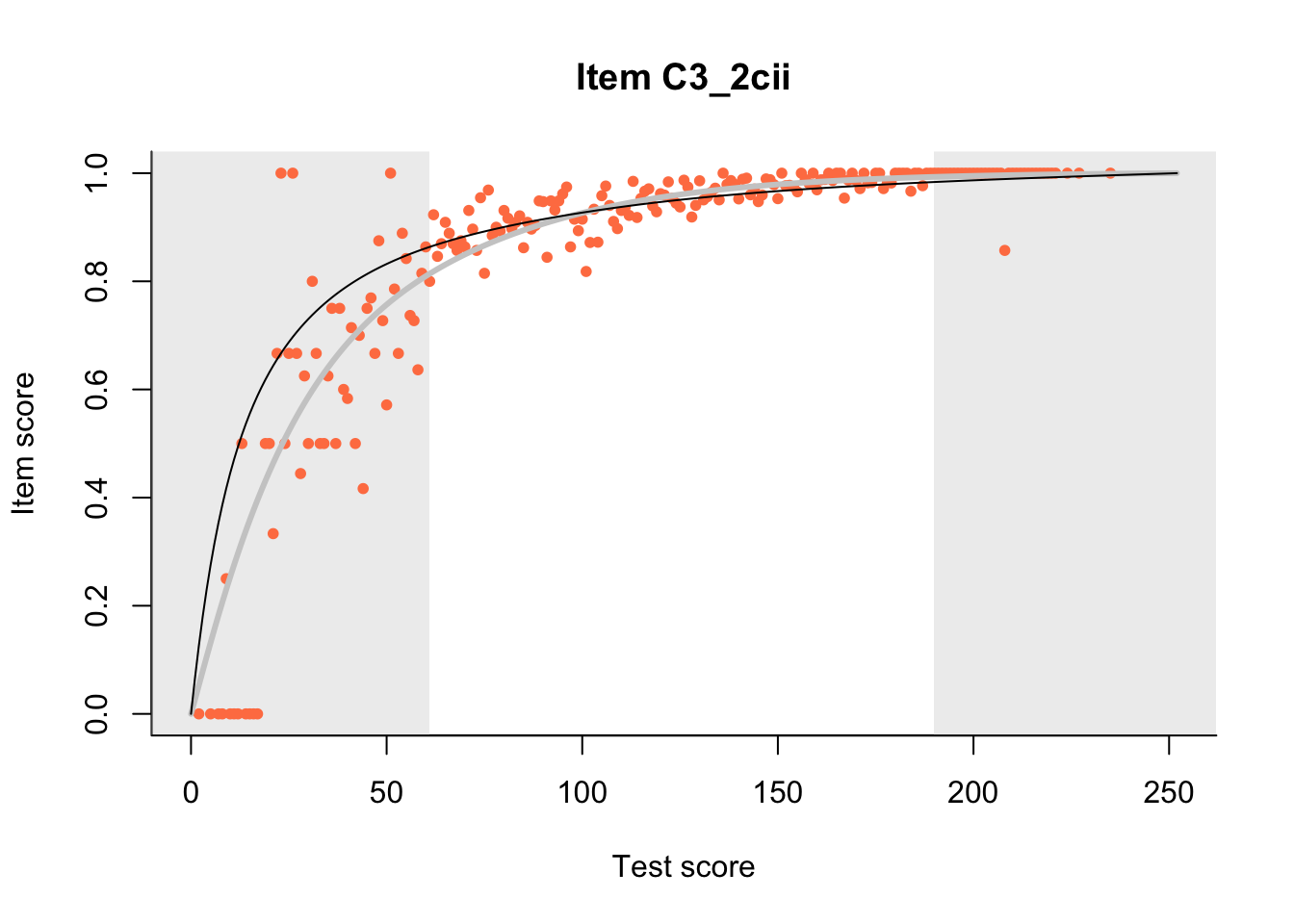
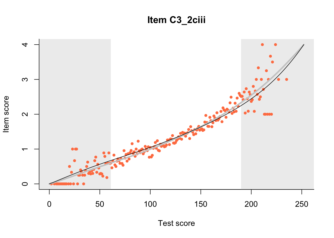
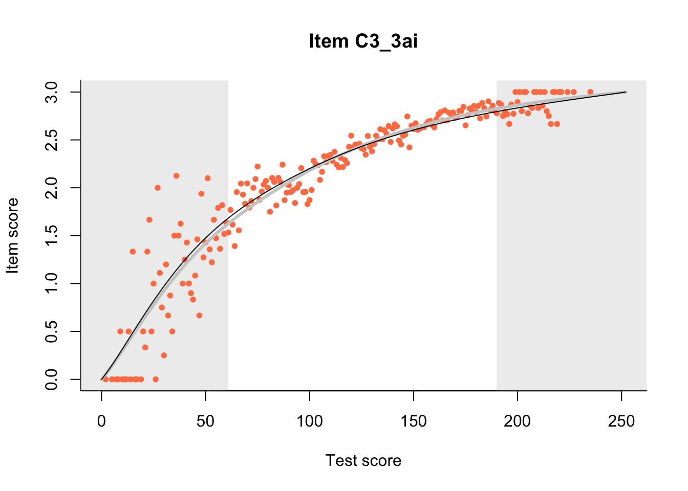
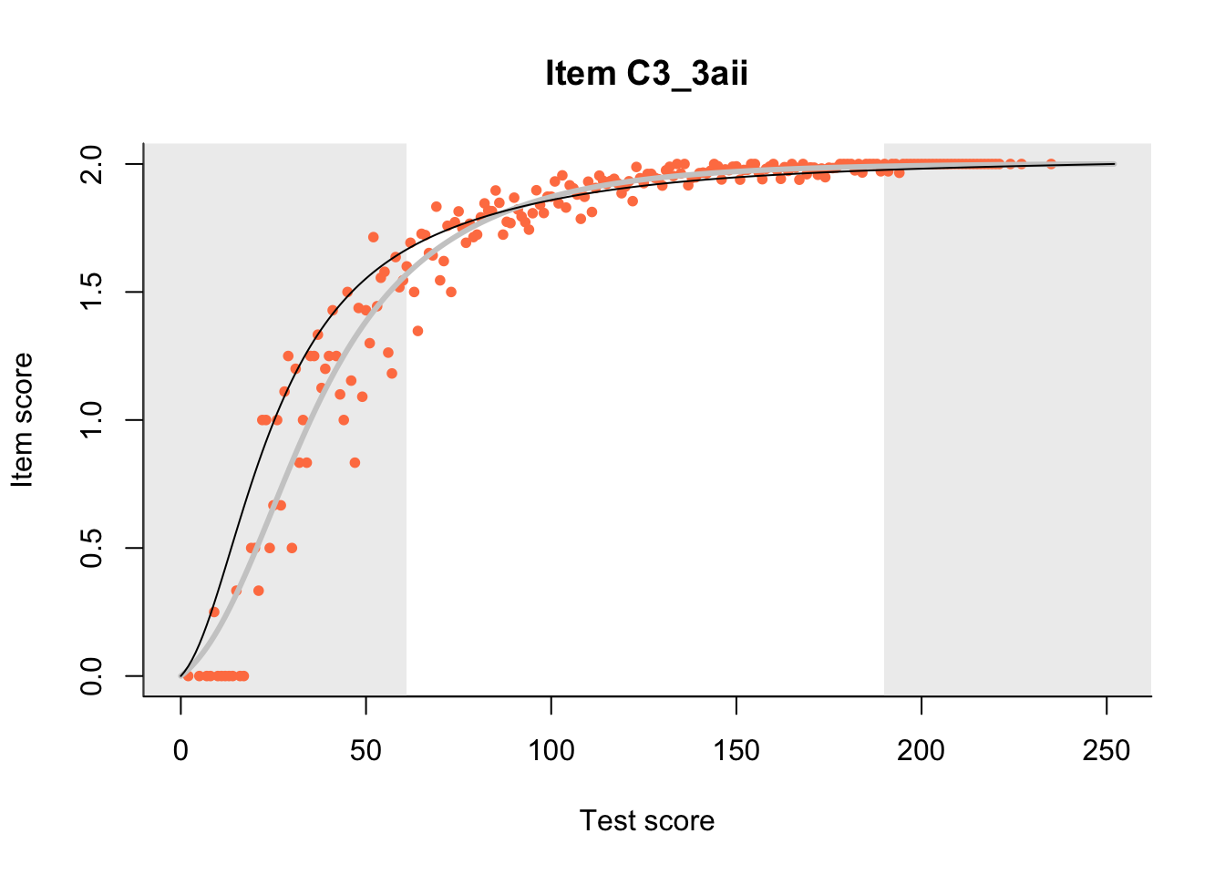
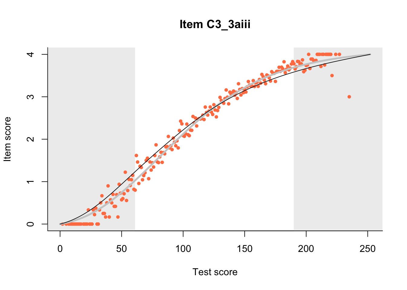
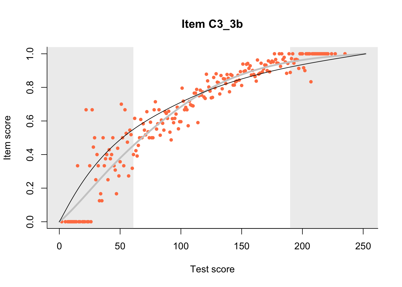
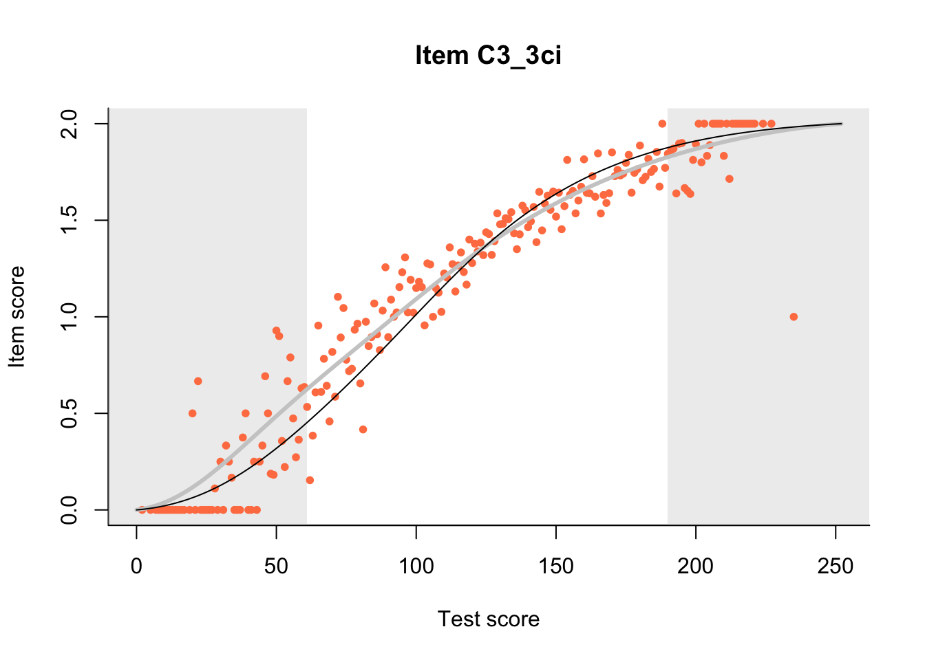
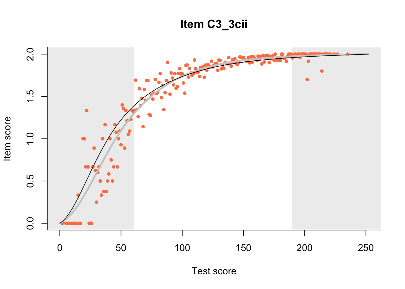
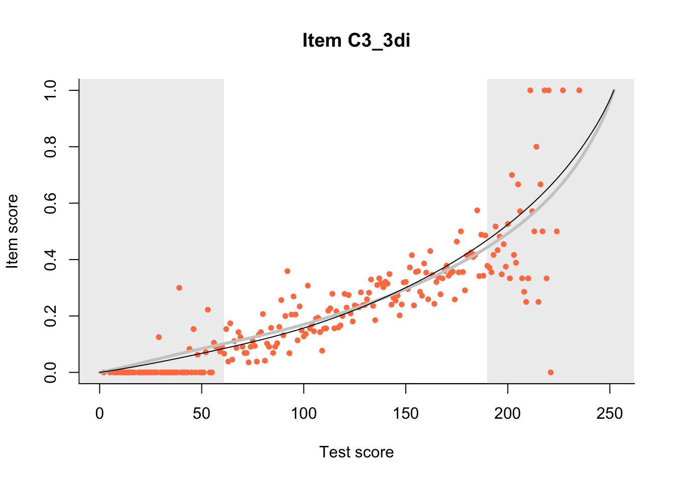
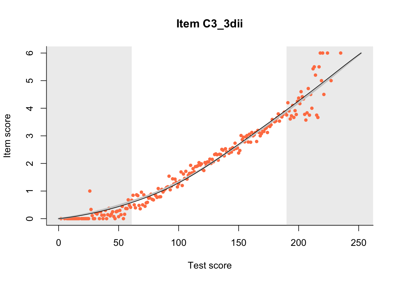
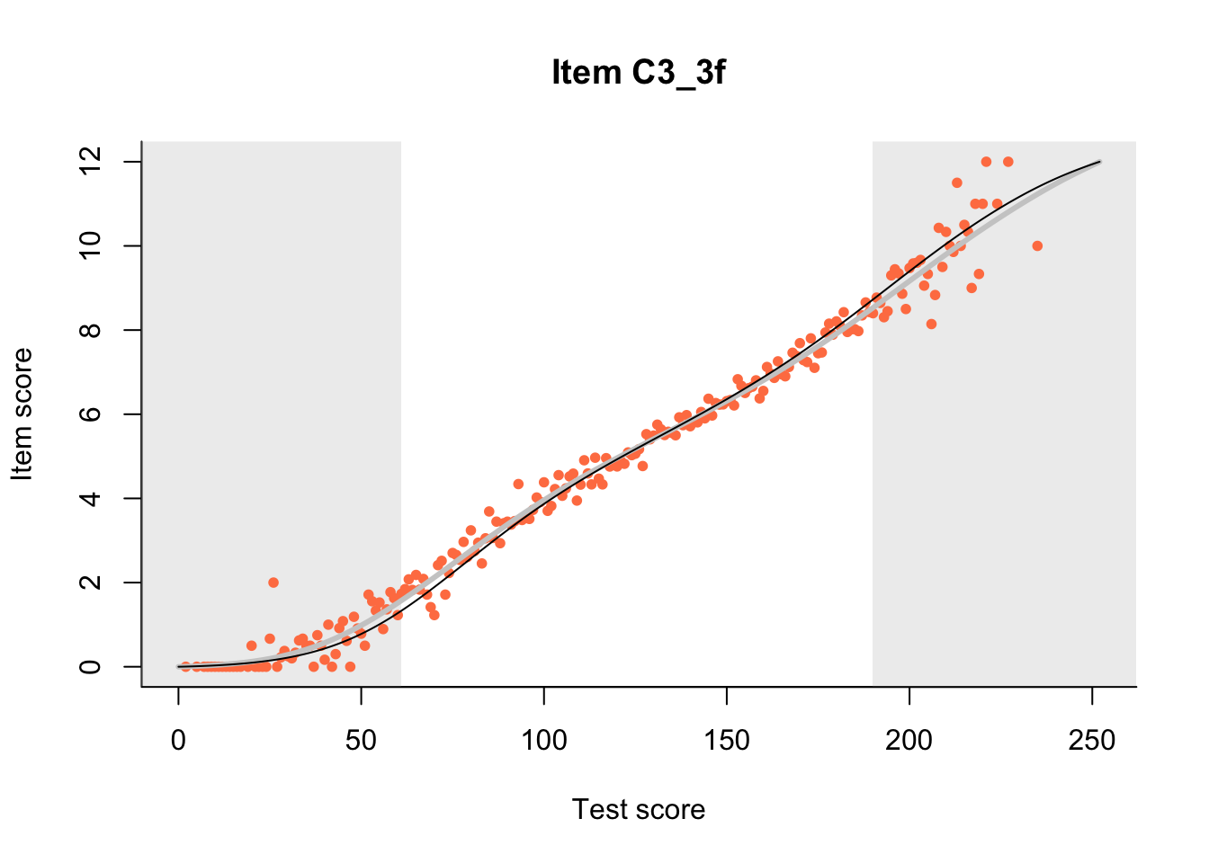
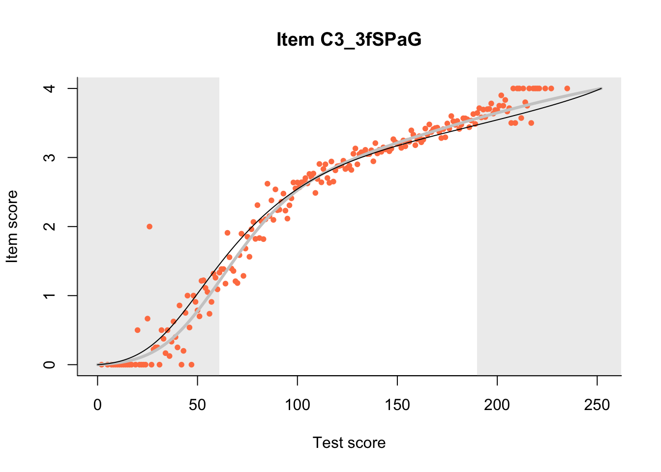
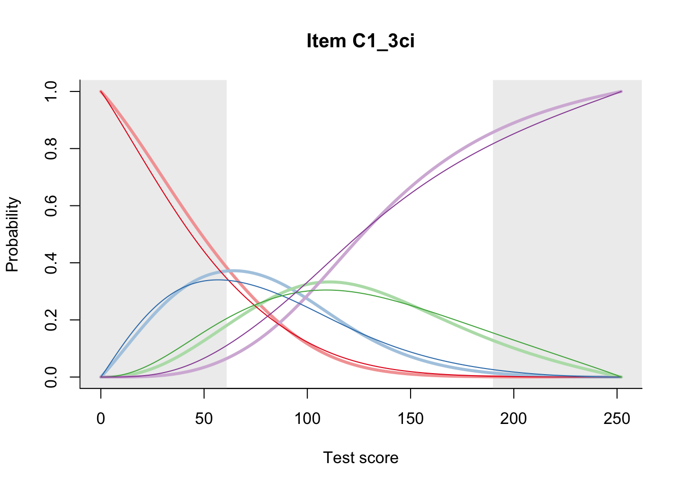
27.1 Expected Score Curves

The Rasch model is shown with a thinner, darker line. The interaction model (unique to dexter) is shown with a thicker, lighter line, and the pink dots show the observed regression.

m = fit_inter(db)
n_items <- nrow(data_summary)
for(i in 1:n_items){
    plot(m, data_summary$Variable[i], show.observed=TRUE)
}

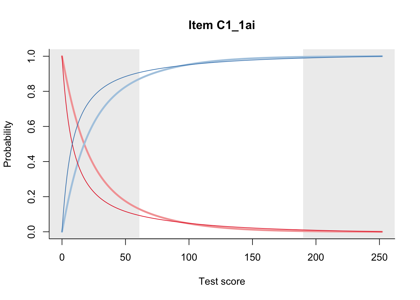
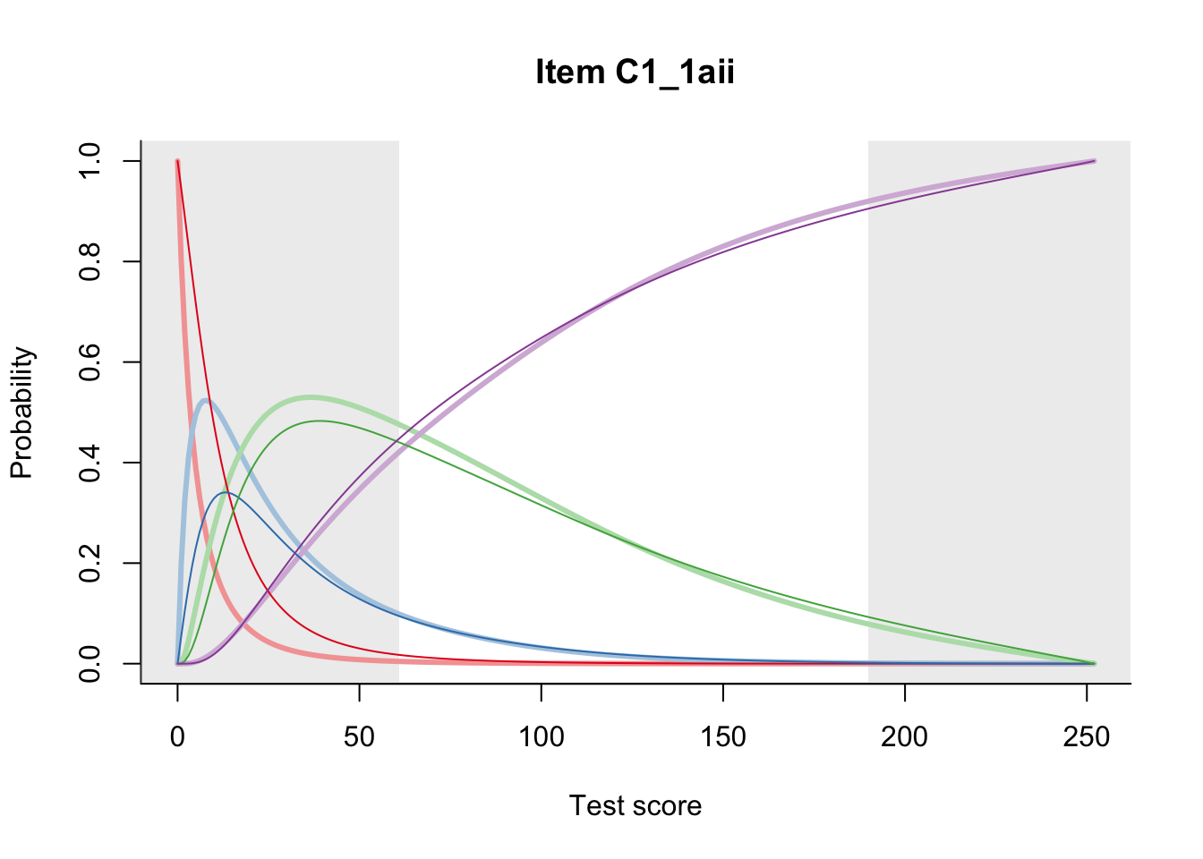
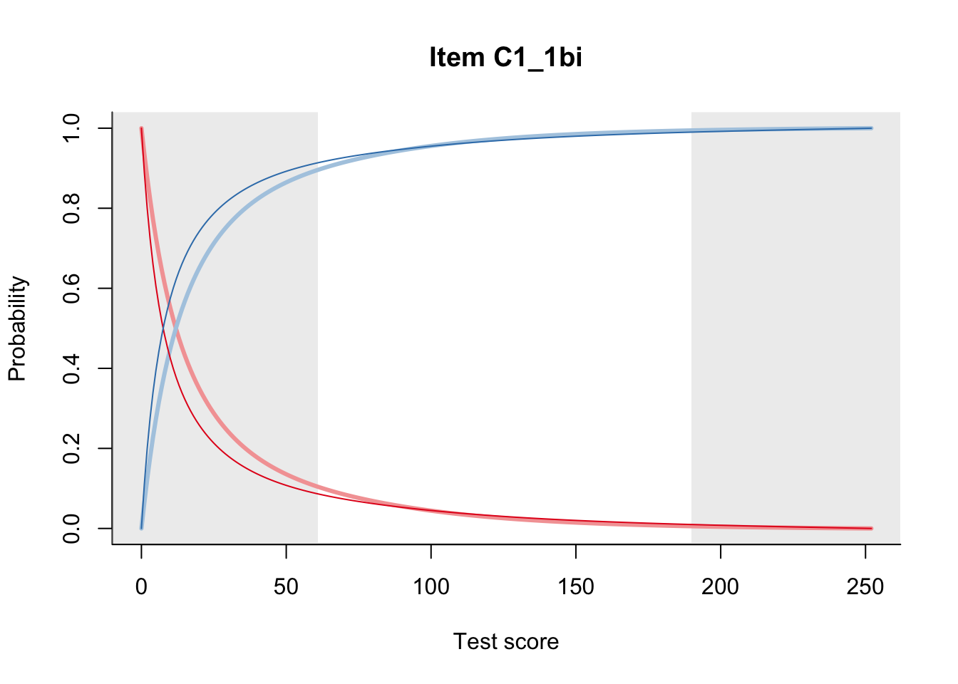
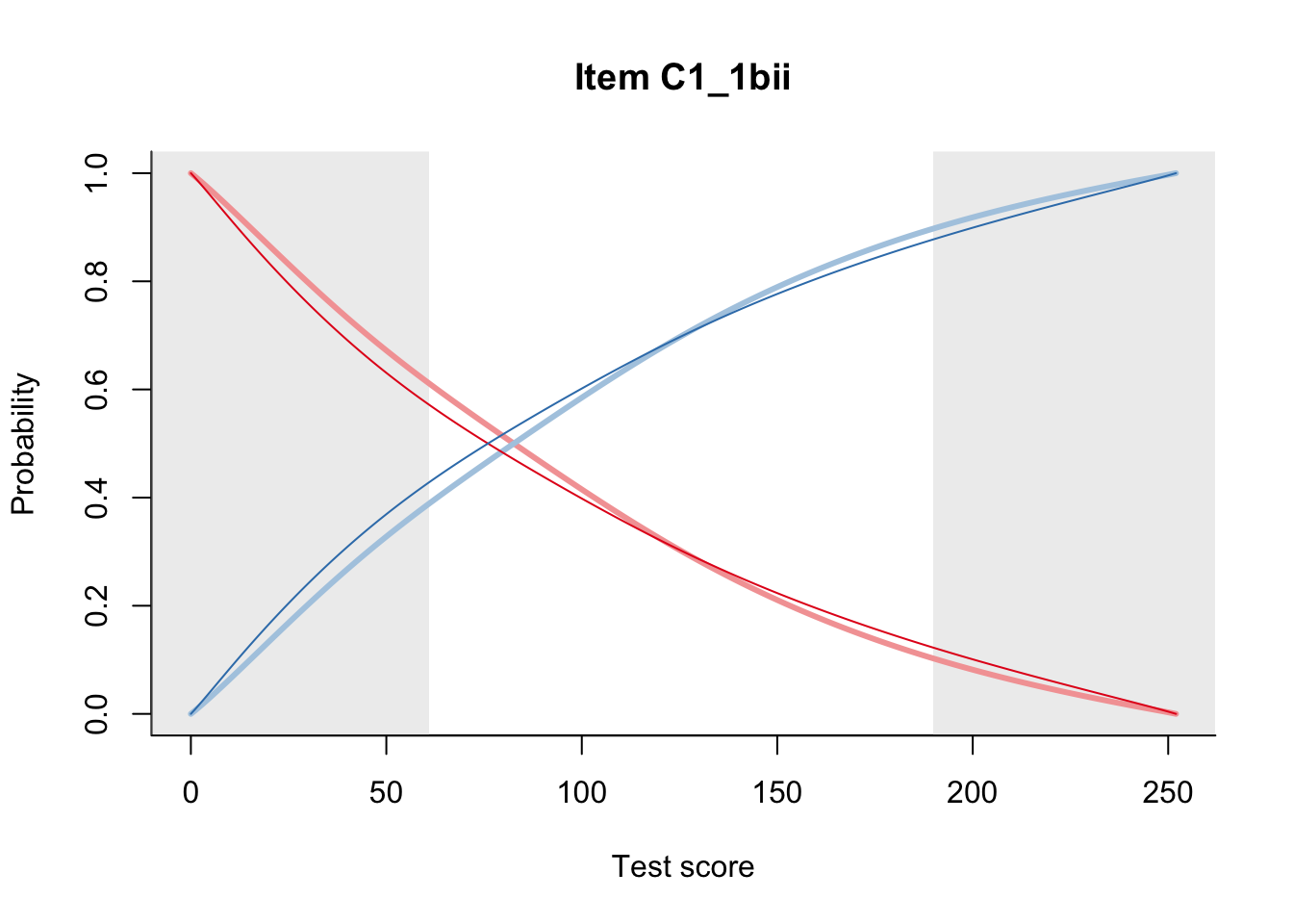
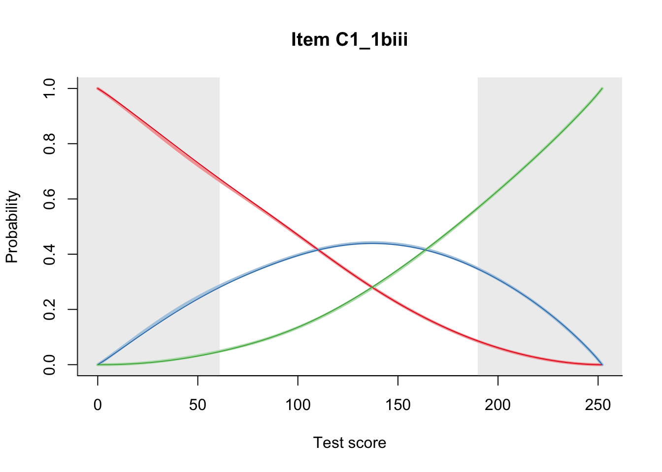
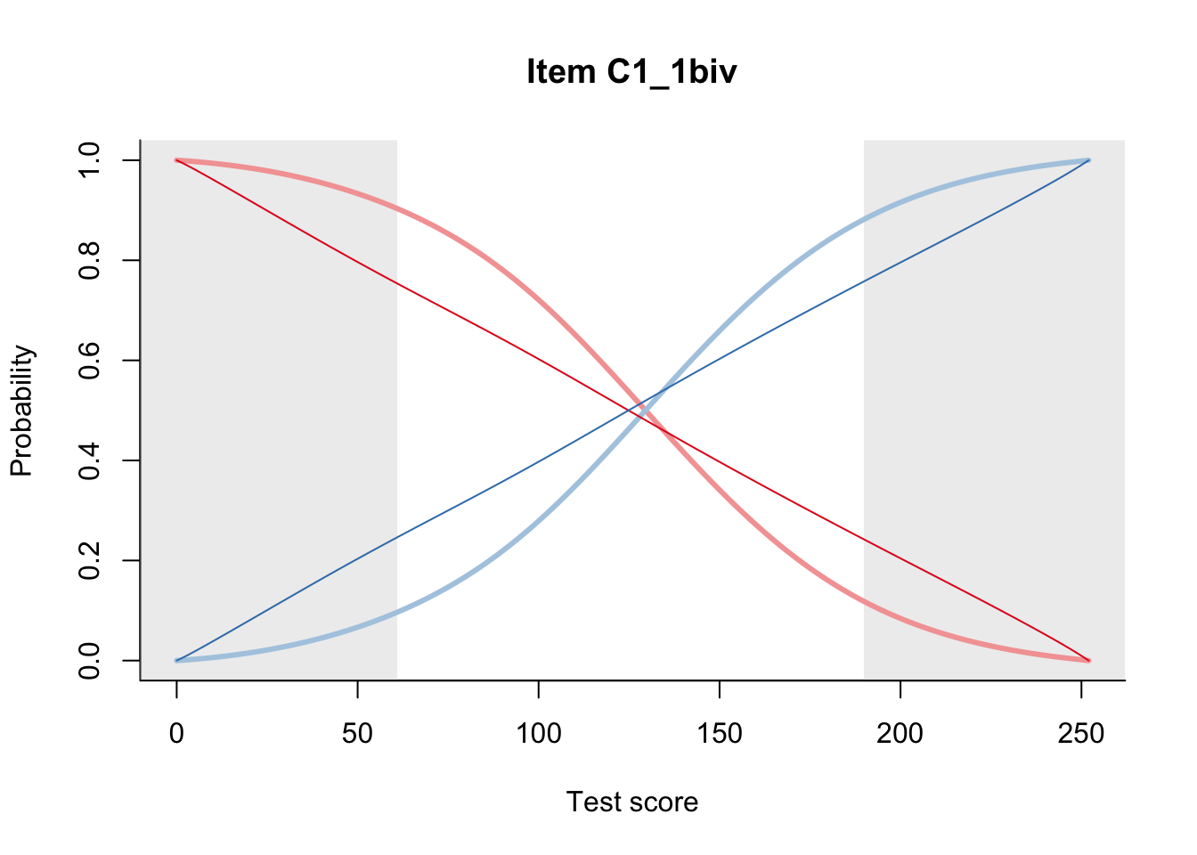
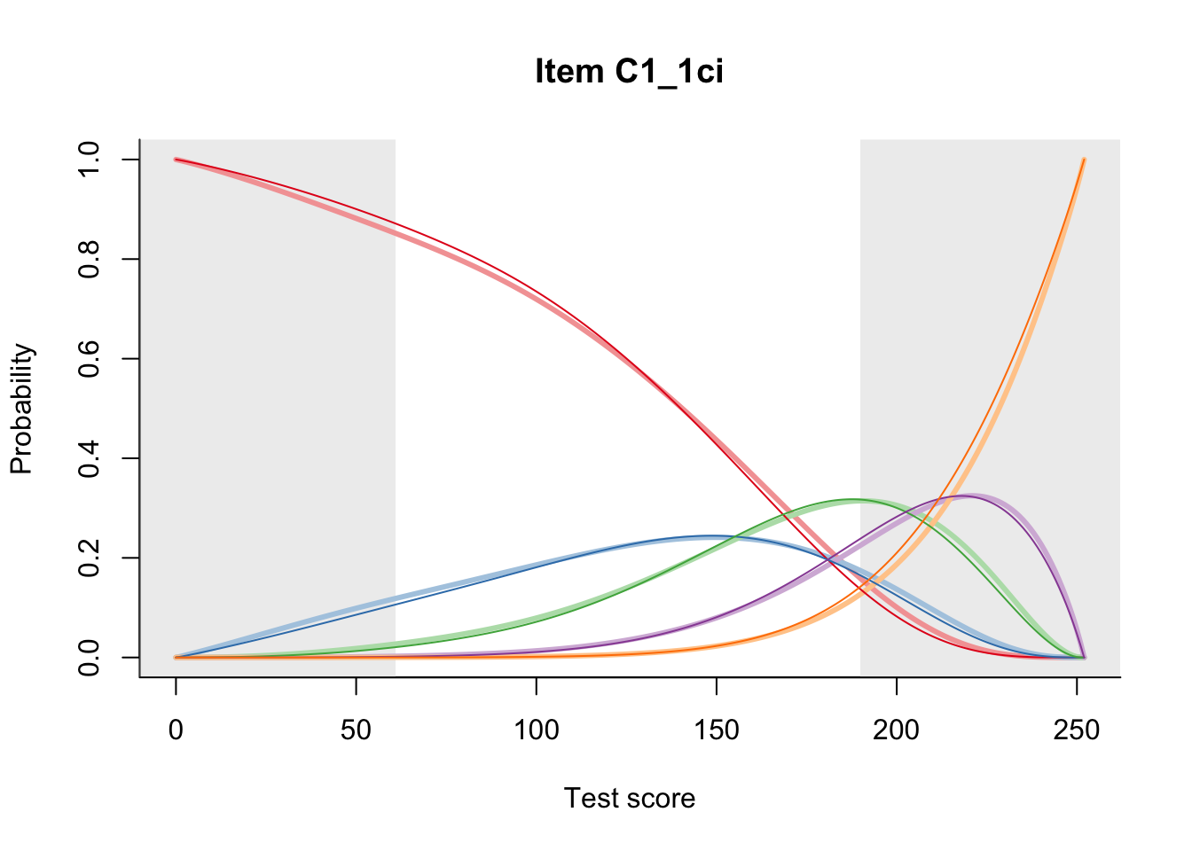
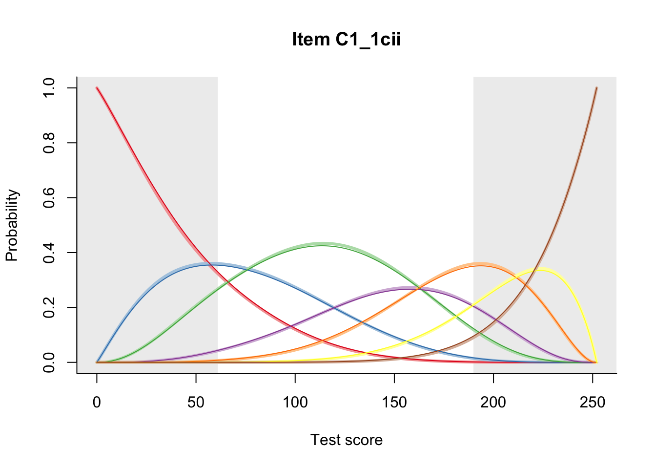
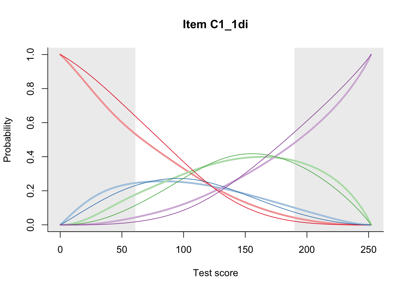
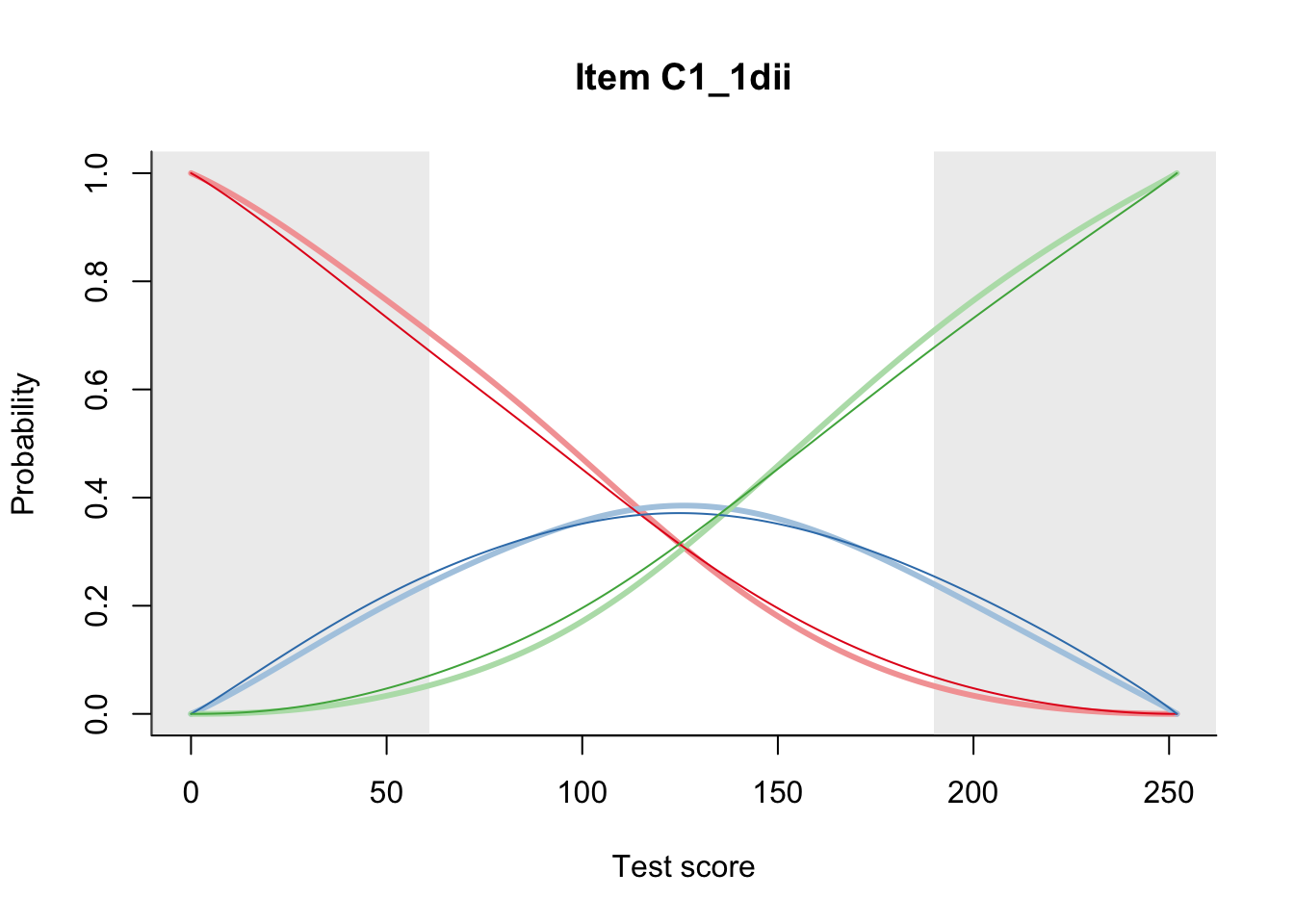
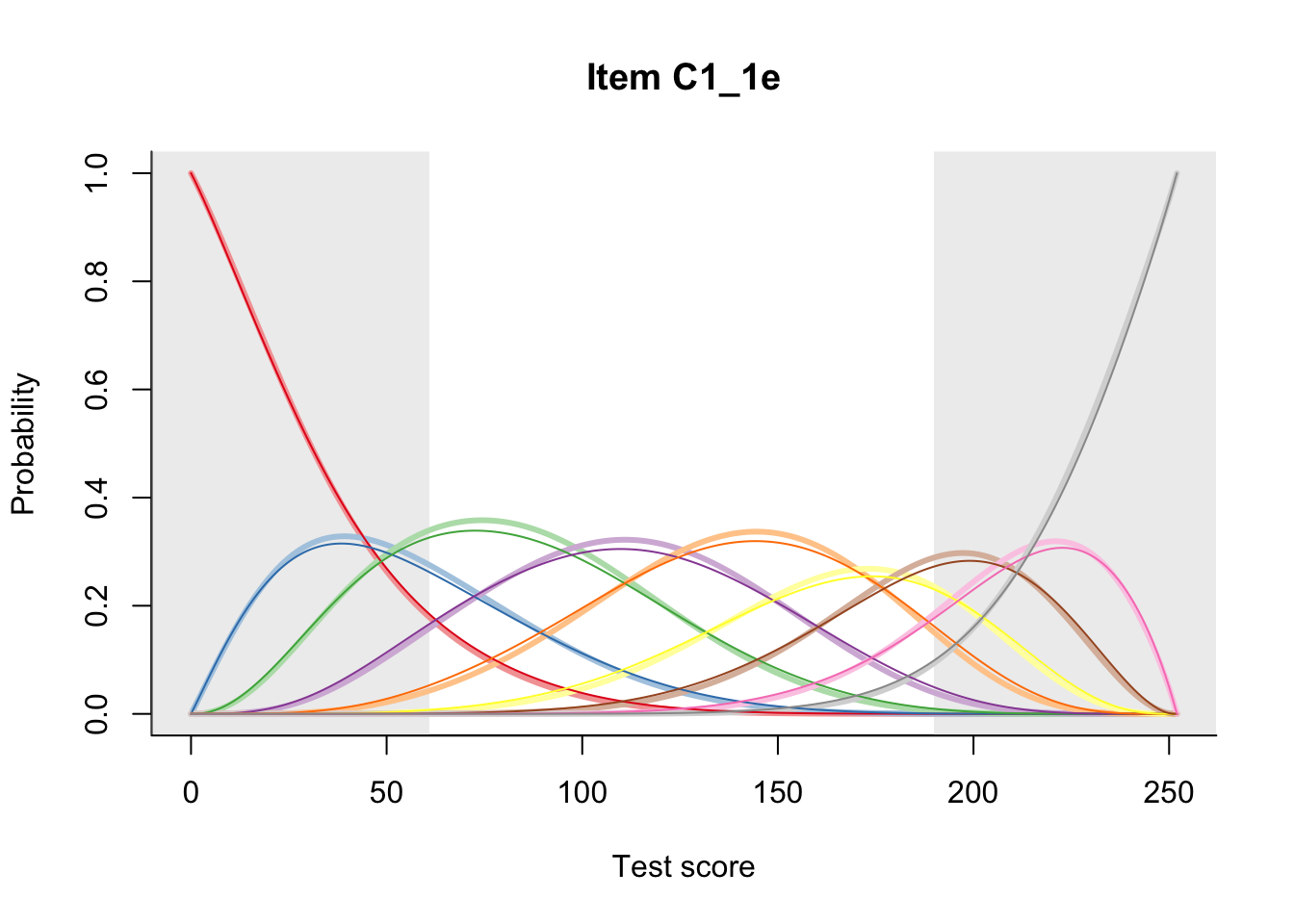
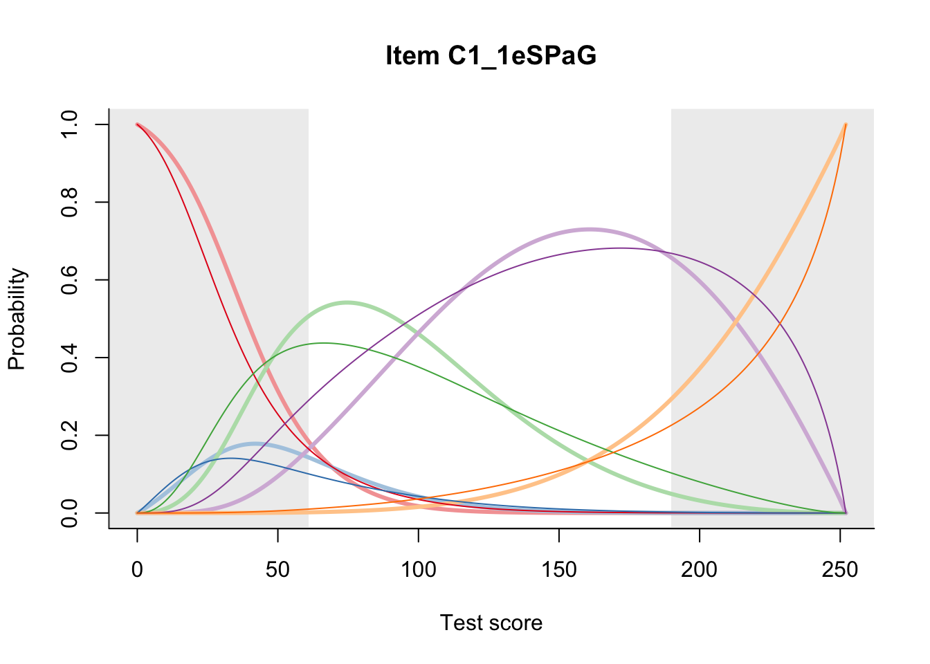
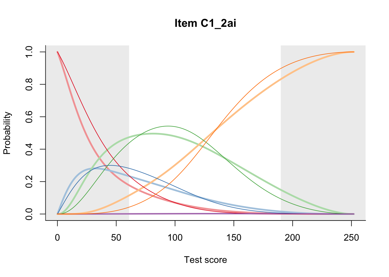
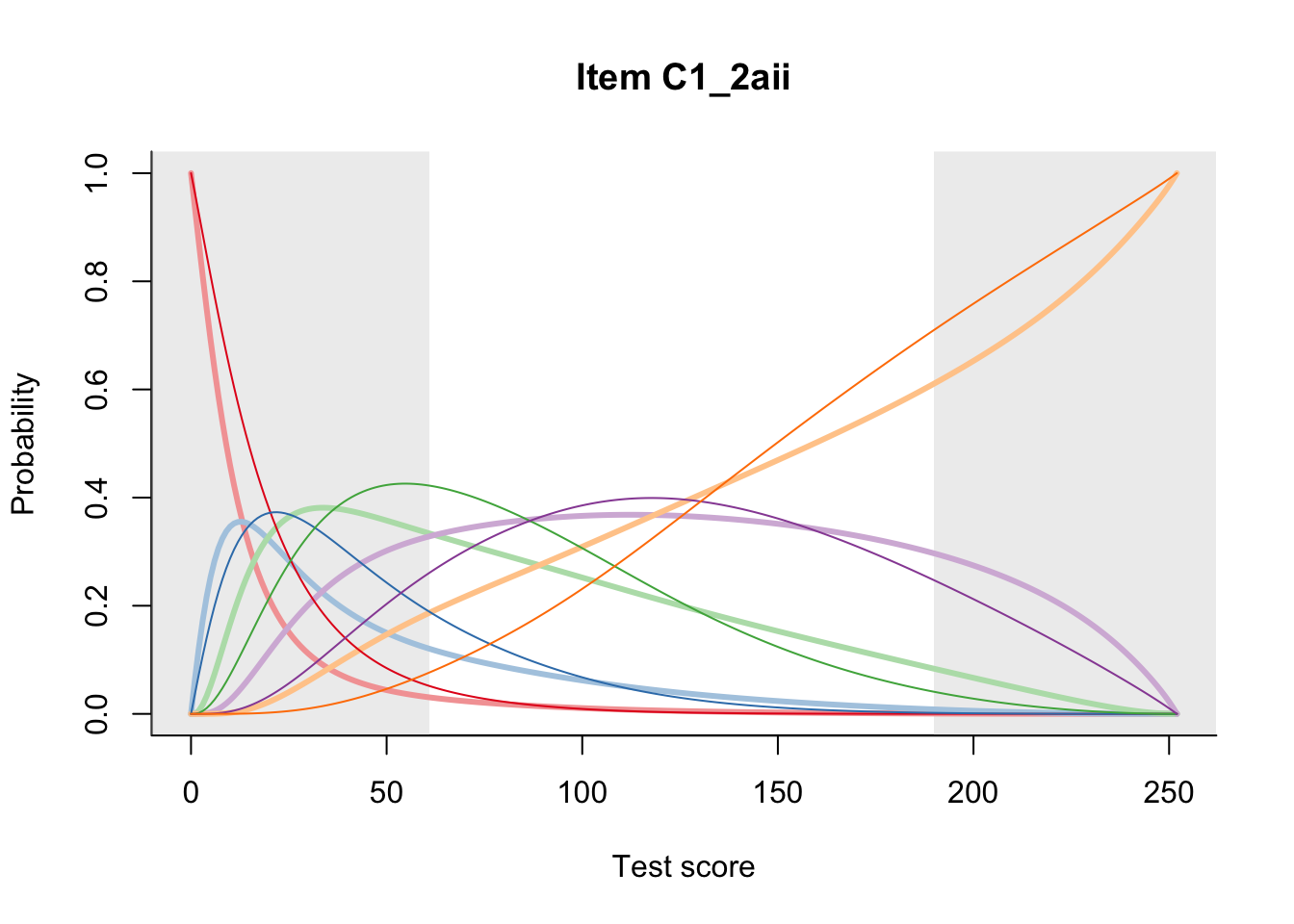
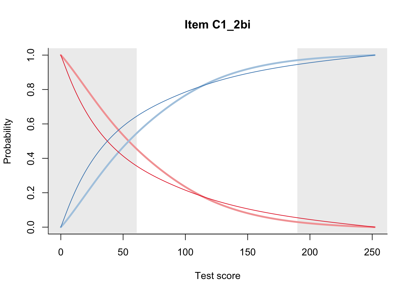
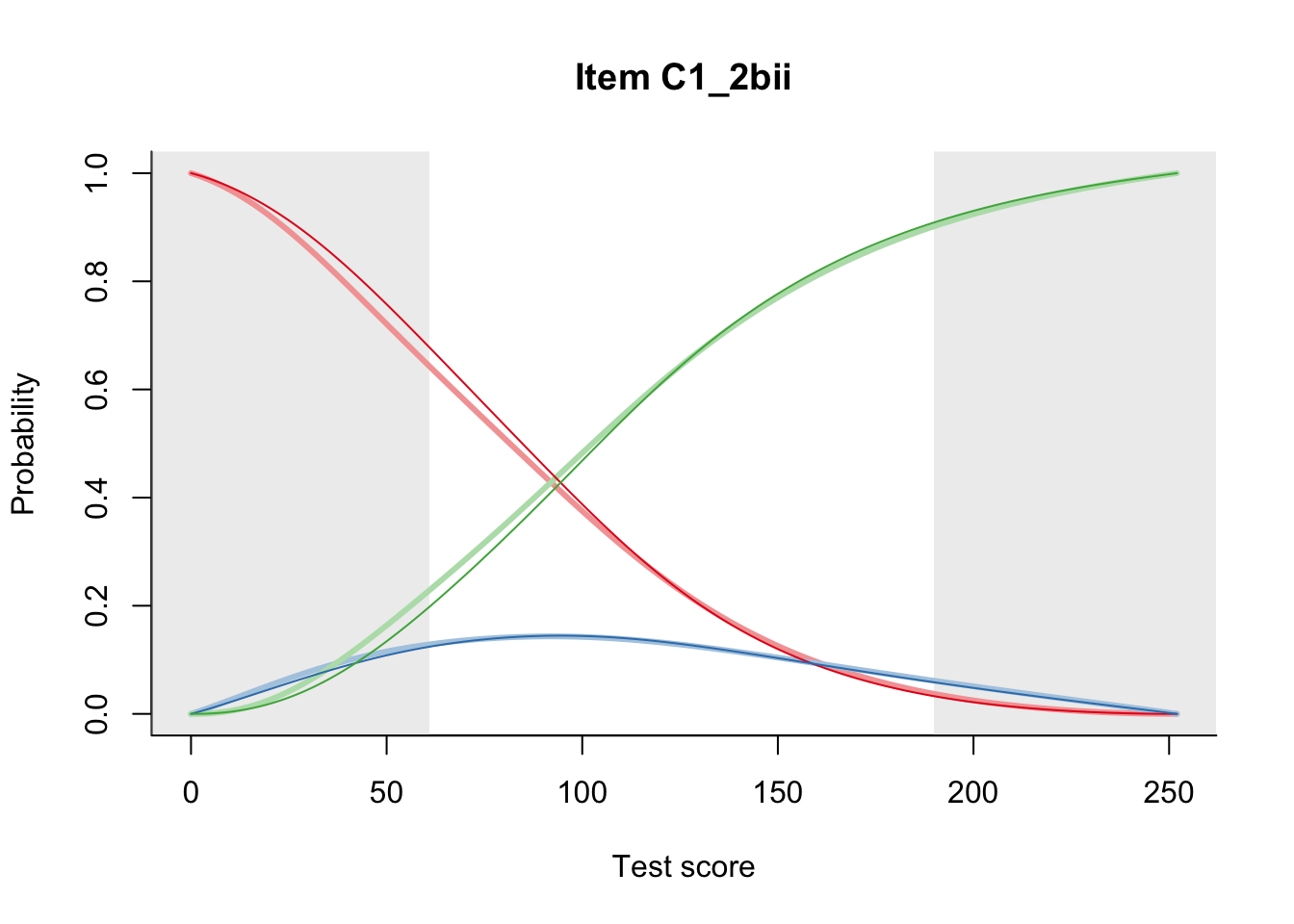
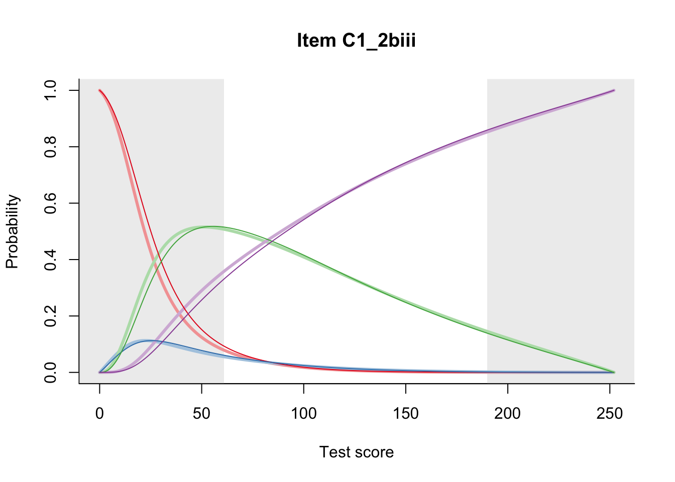
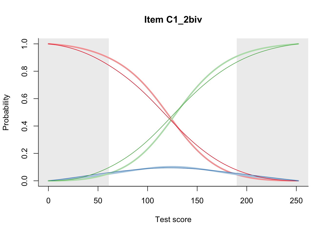
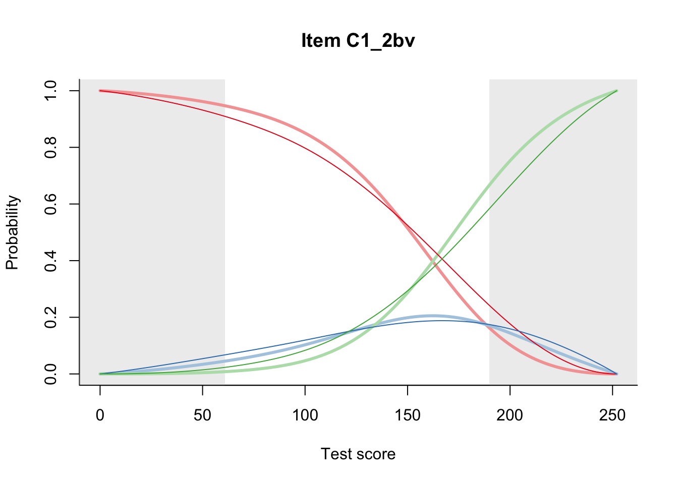
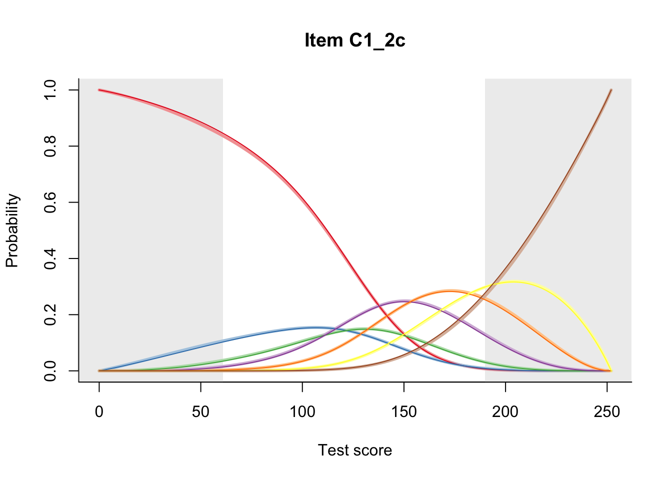
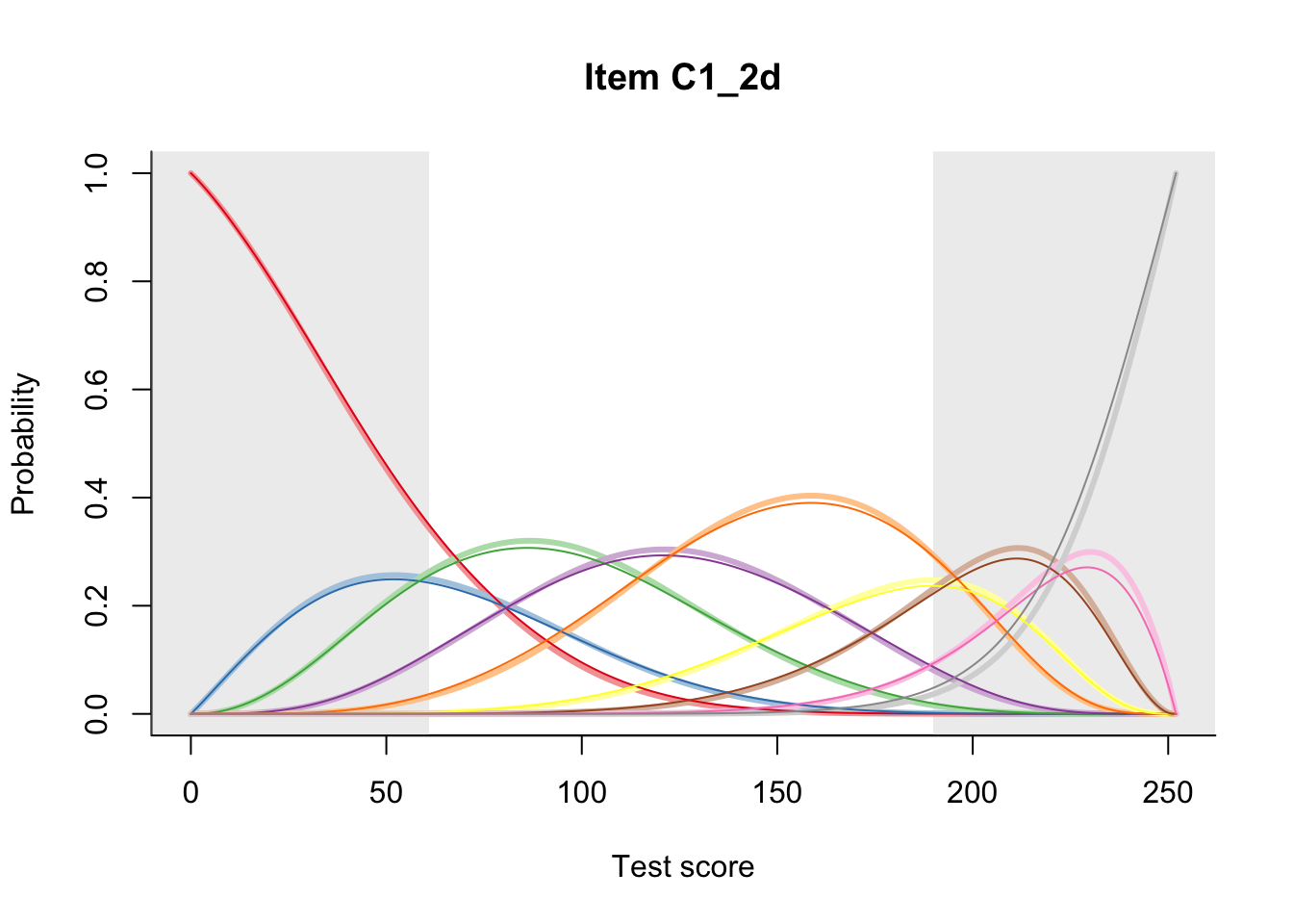
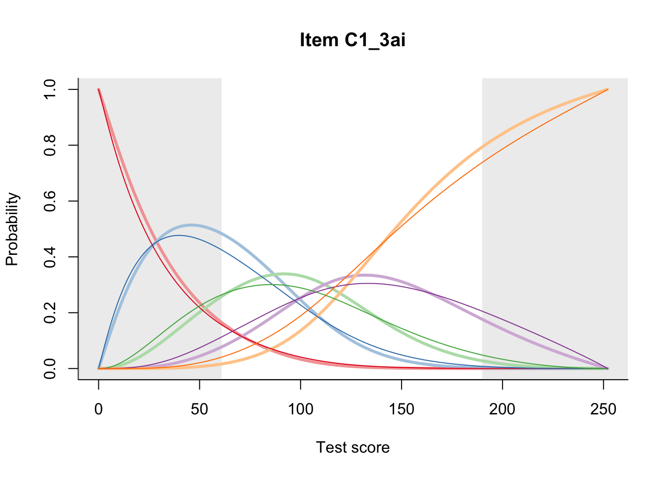
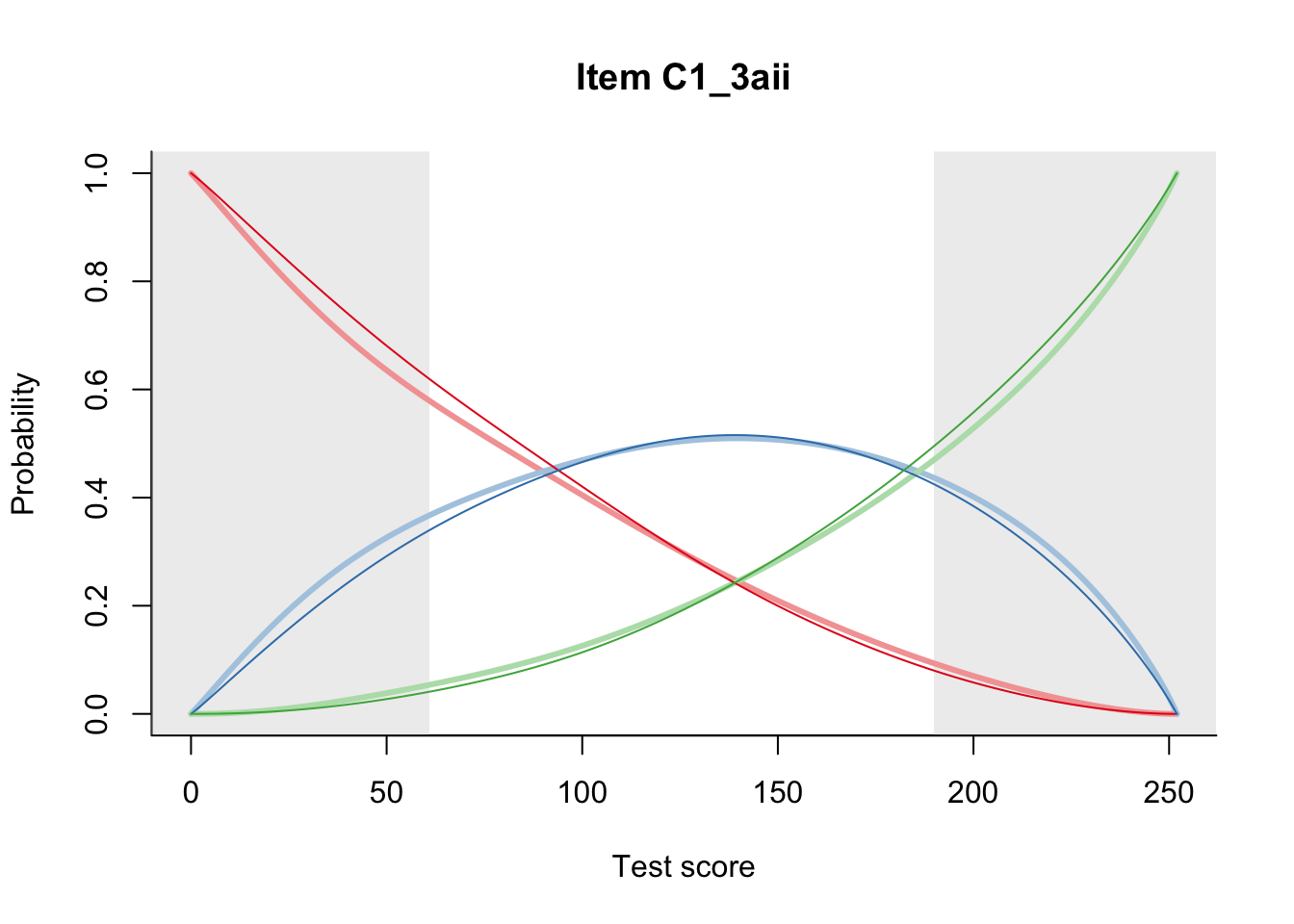
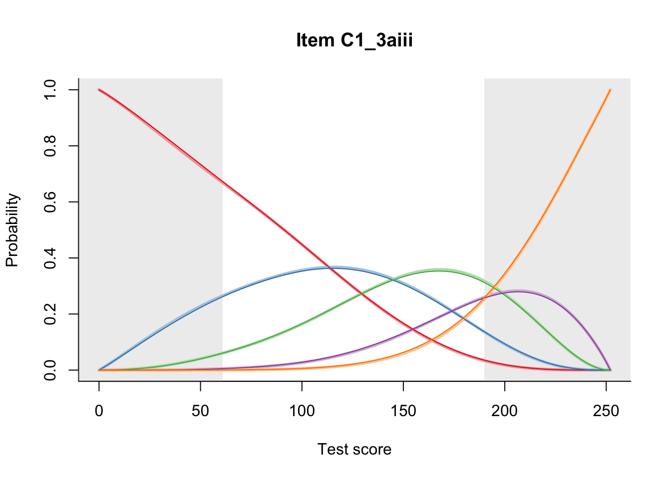
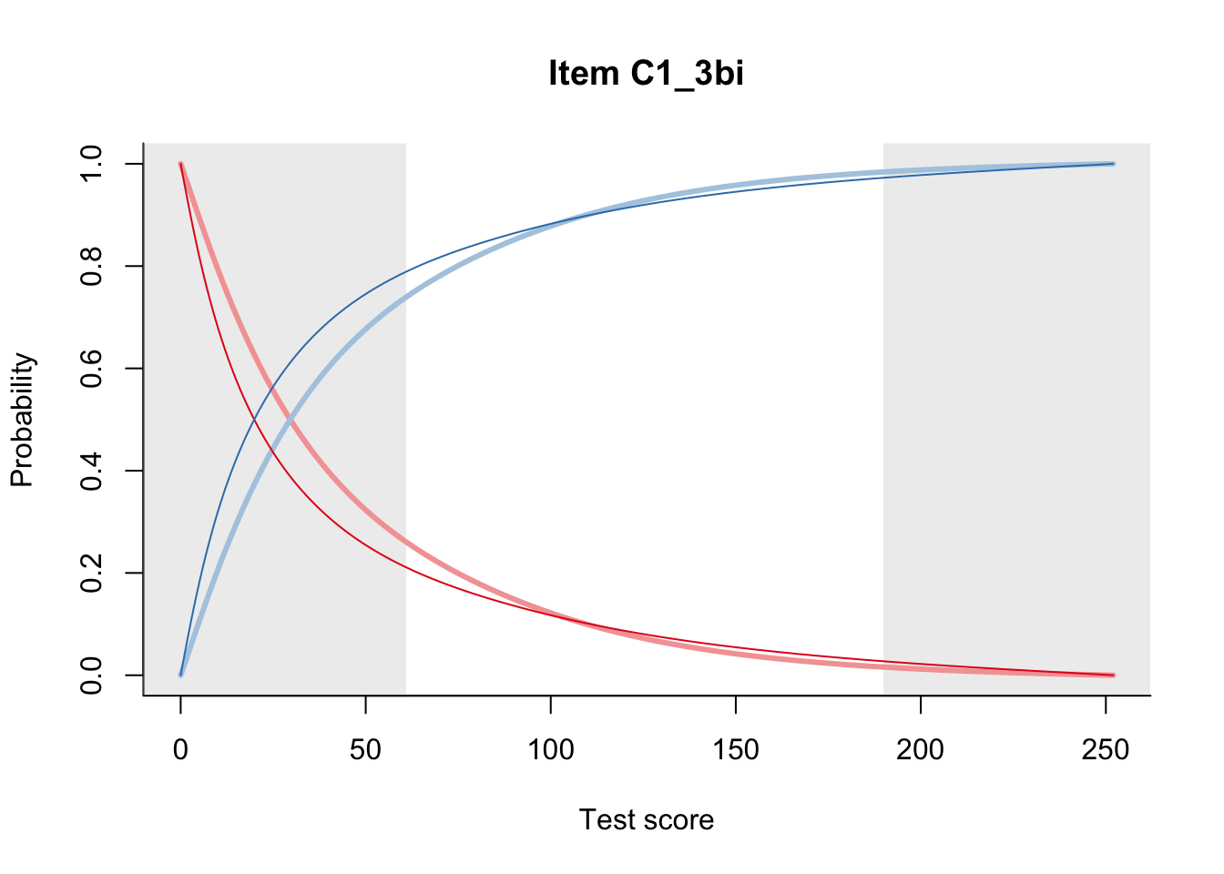
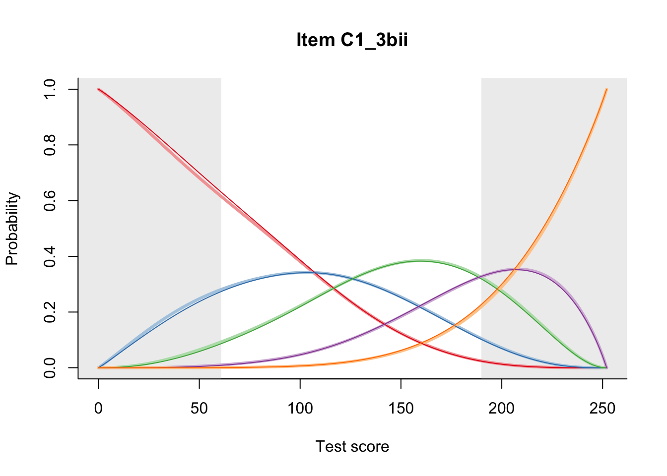
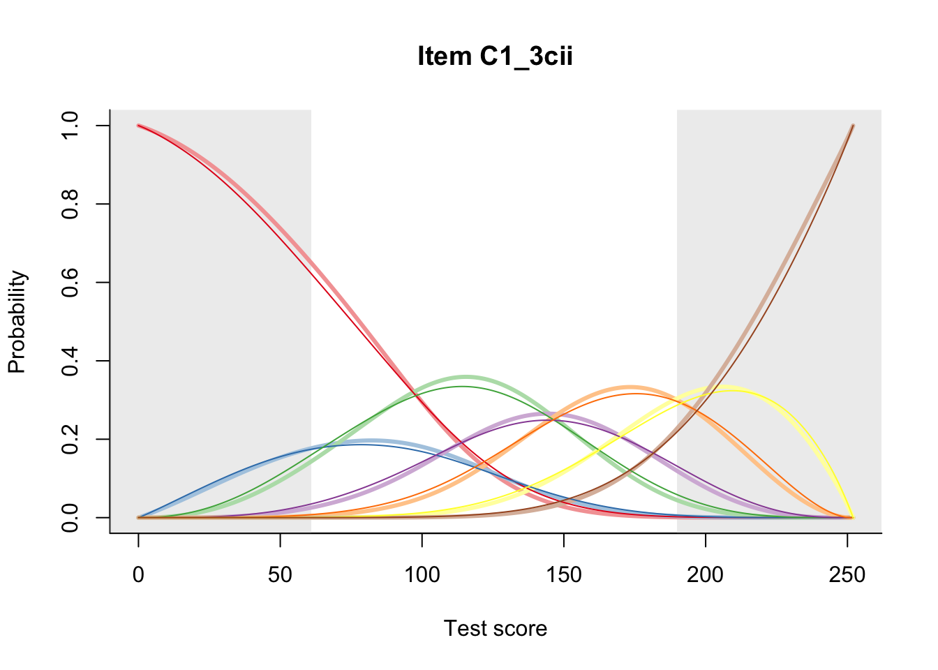
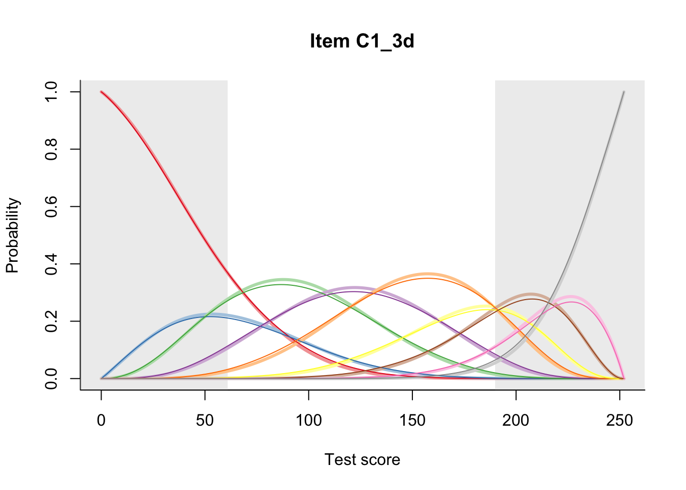
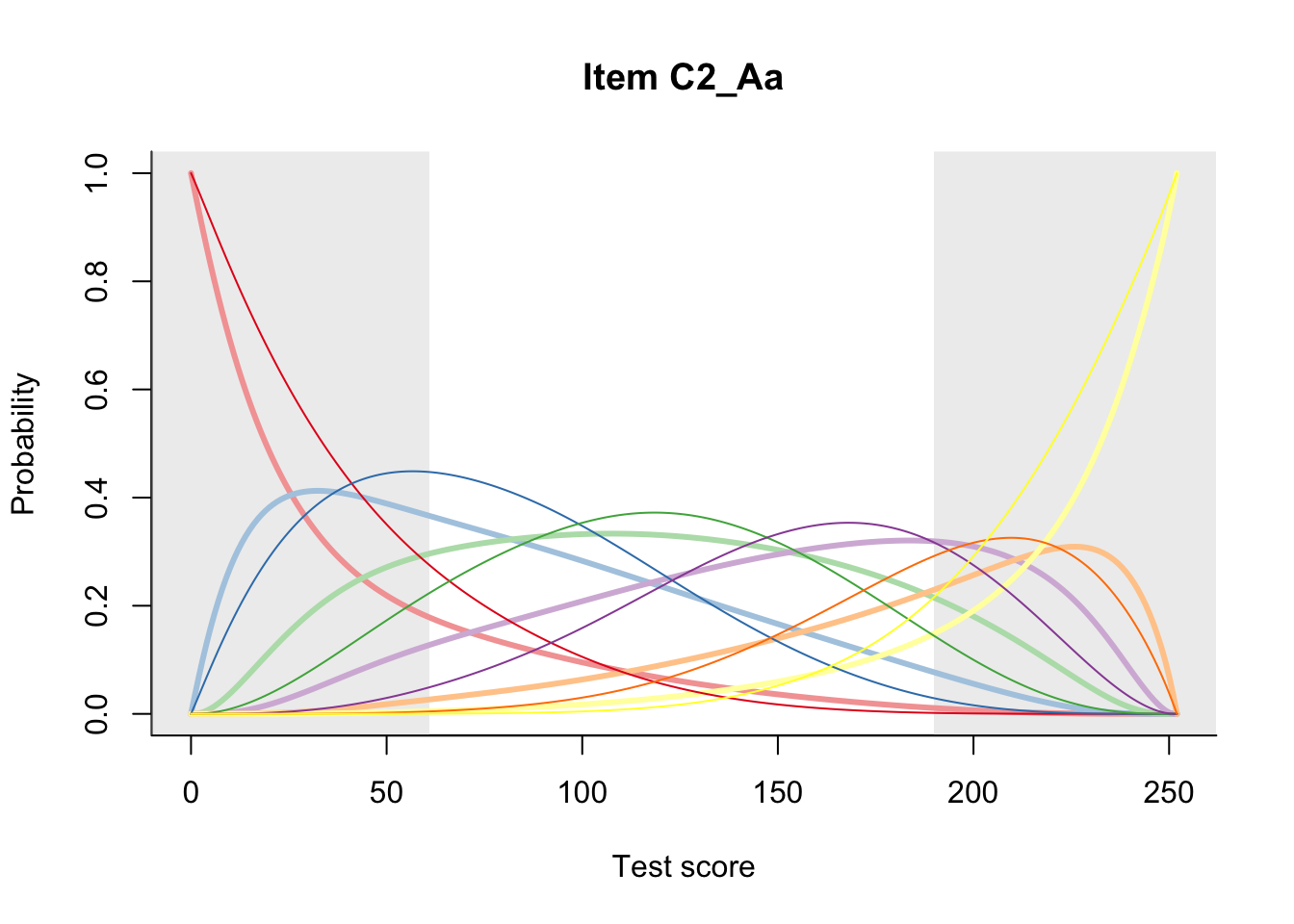
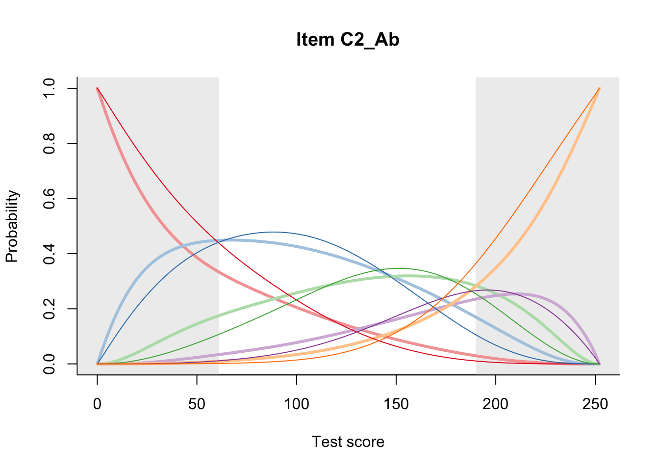
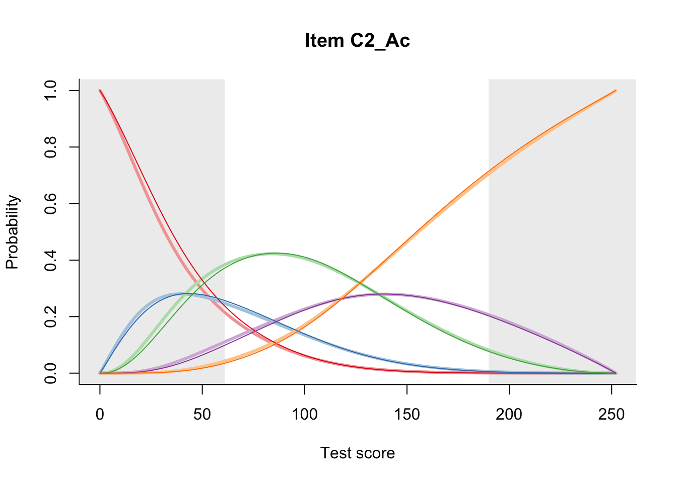
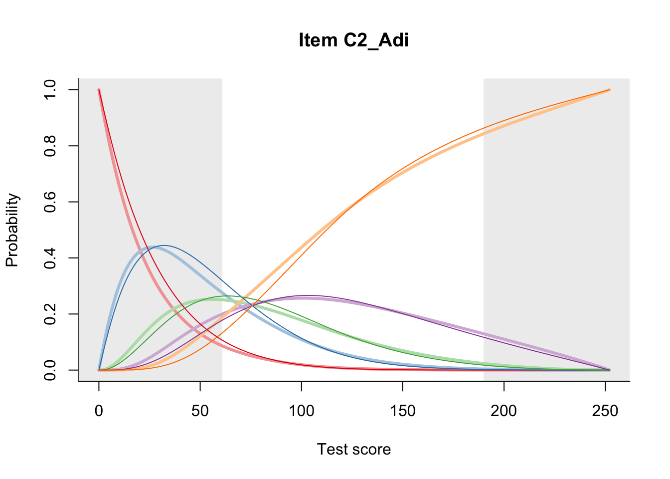
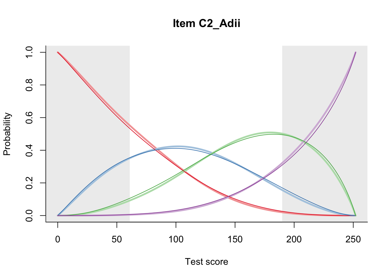
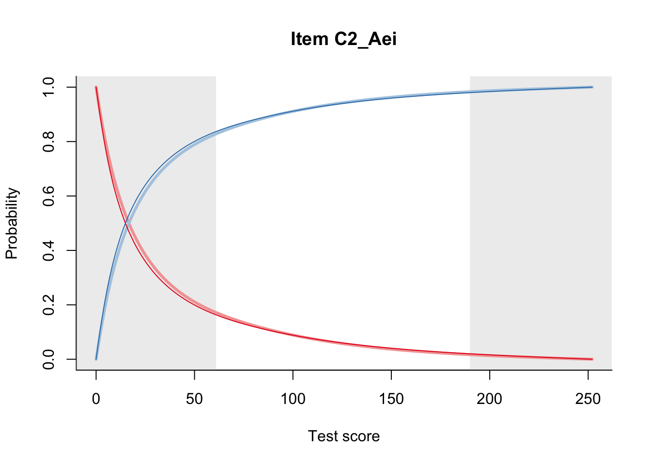
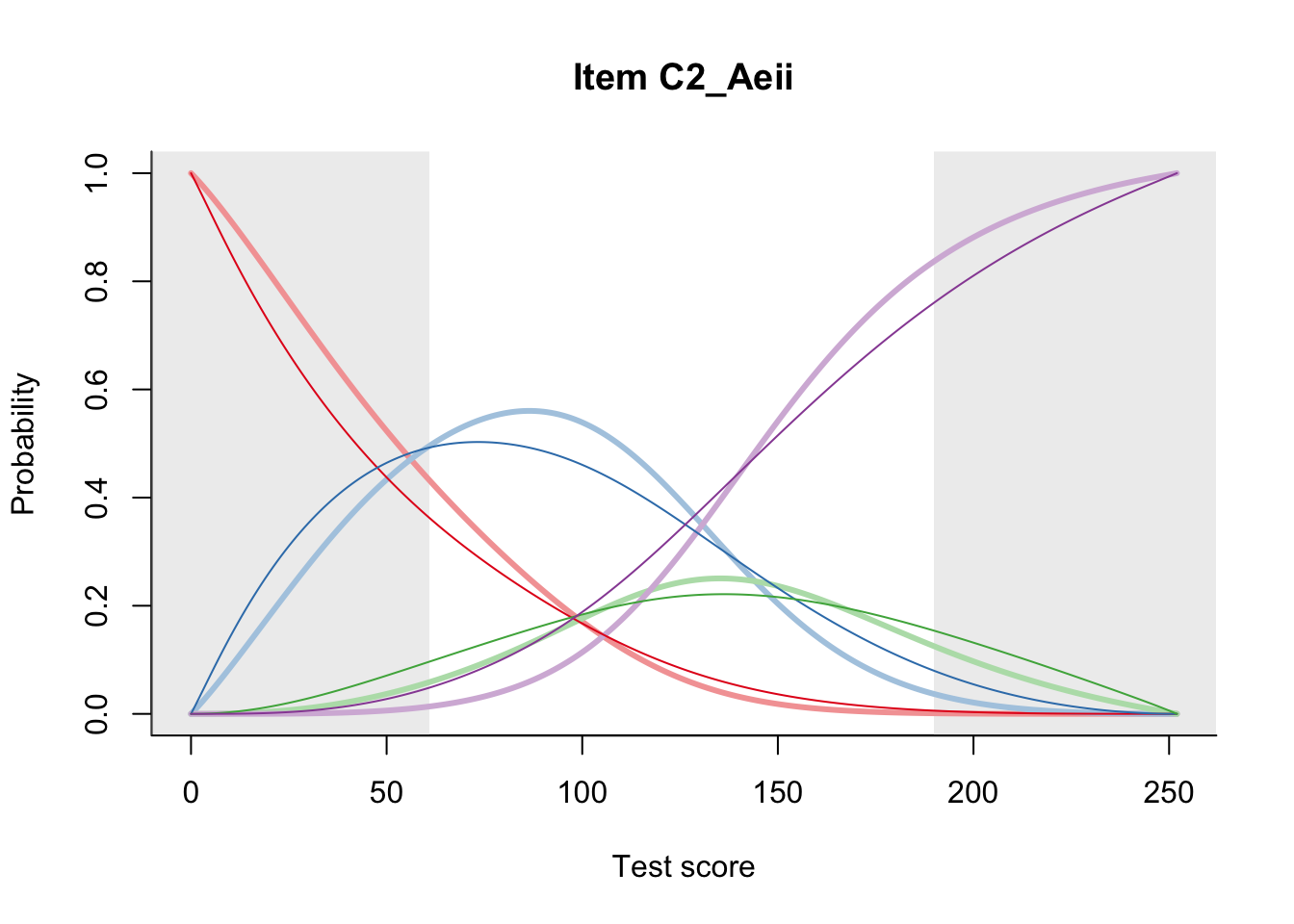
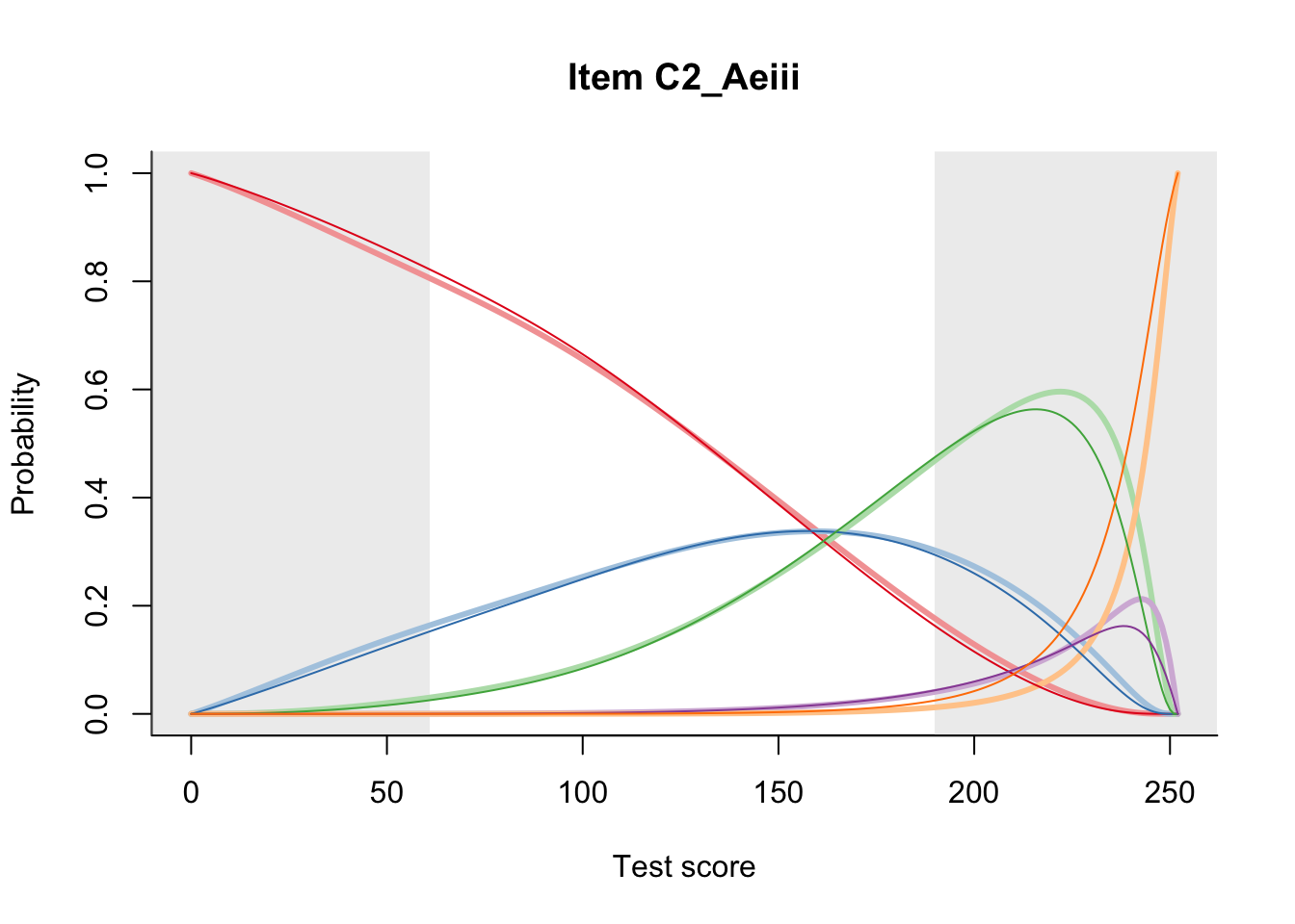
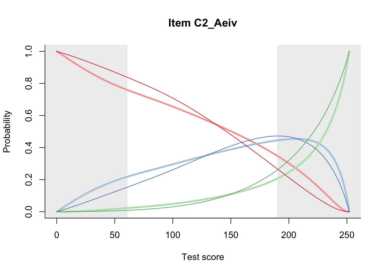
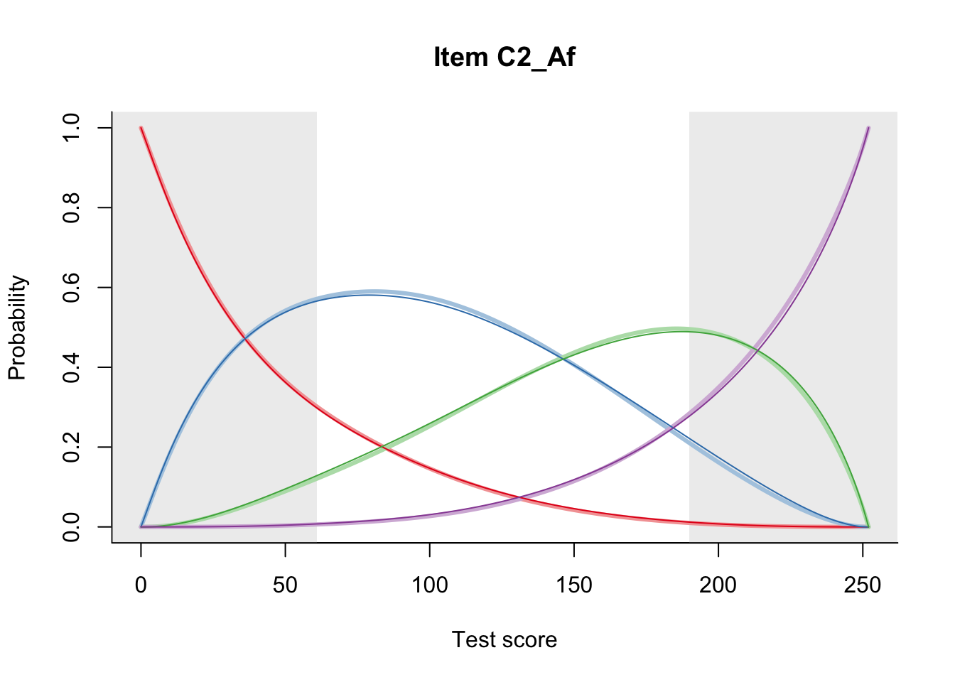
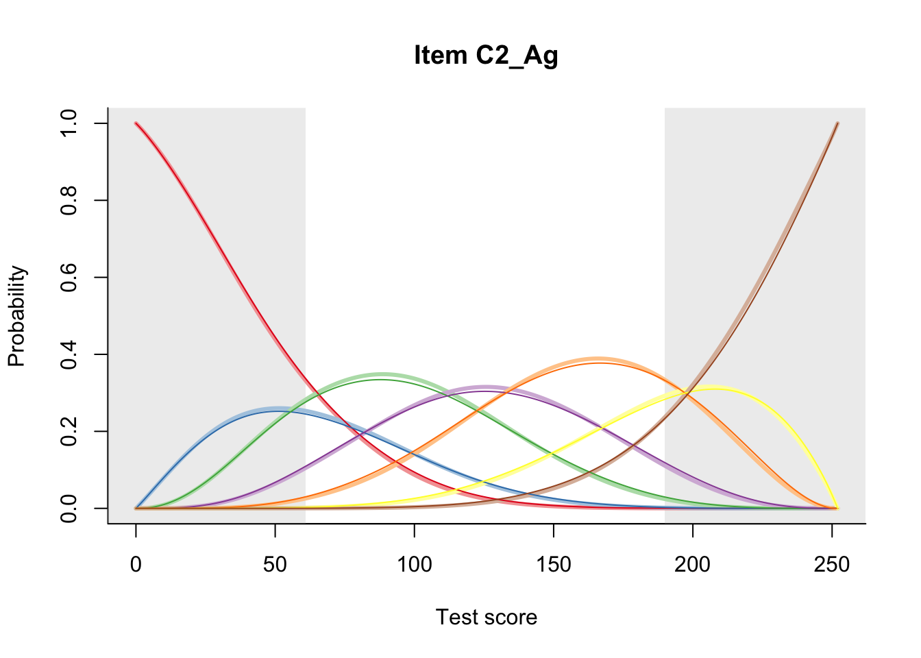
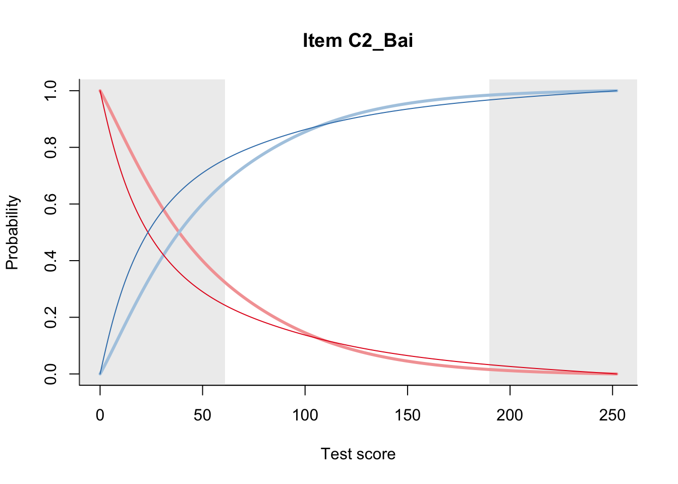
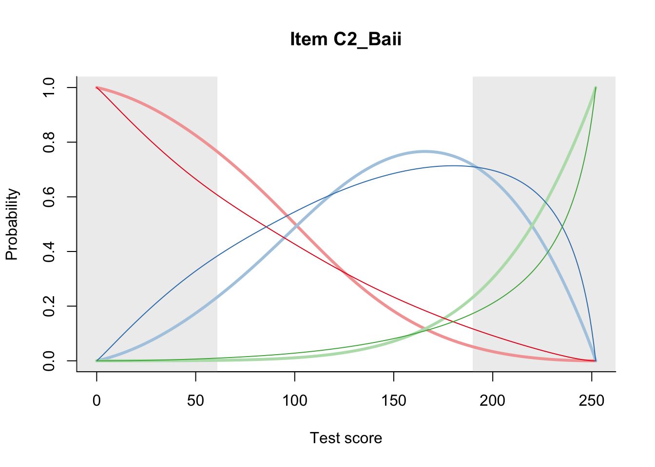
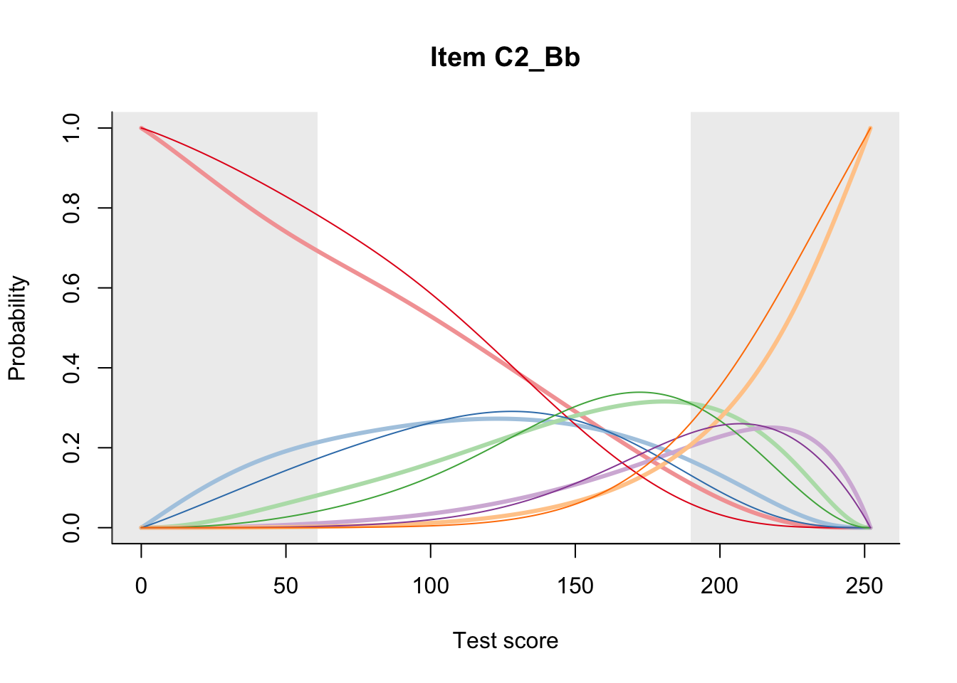
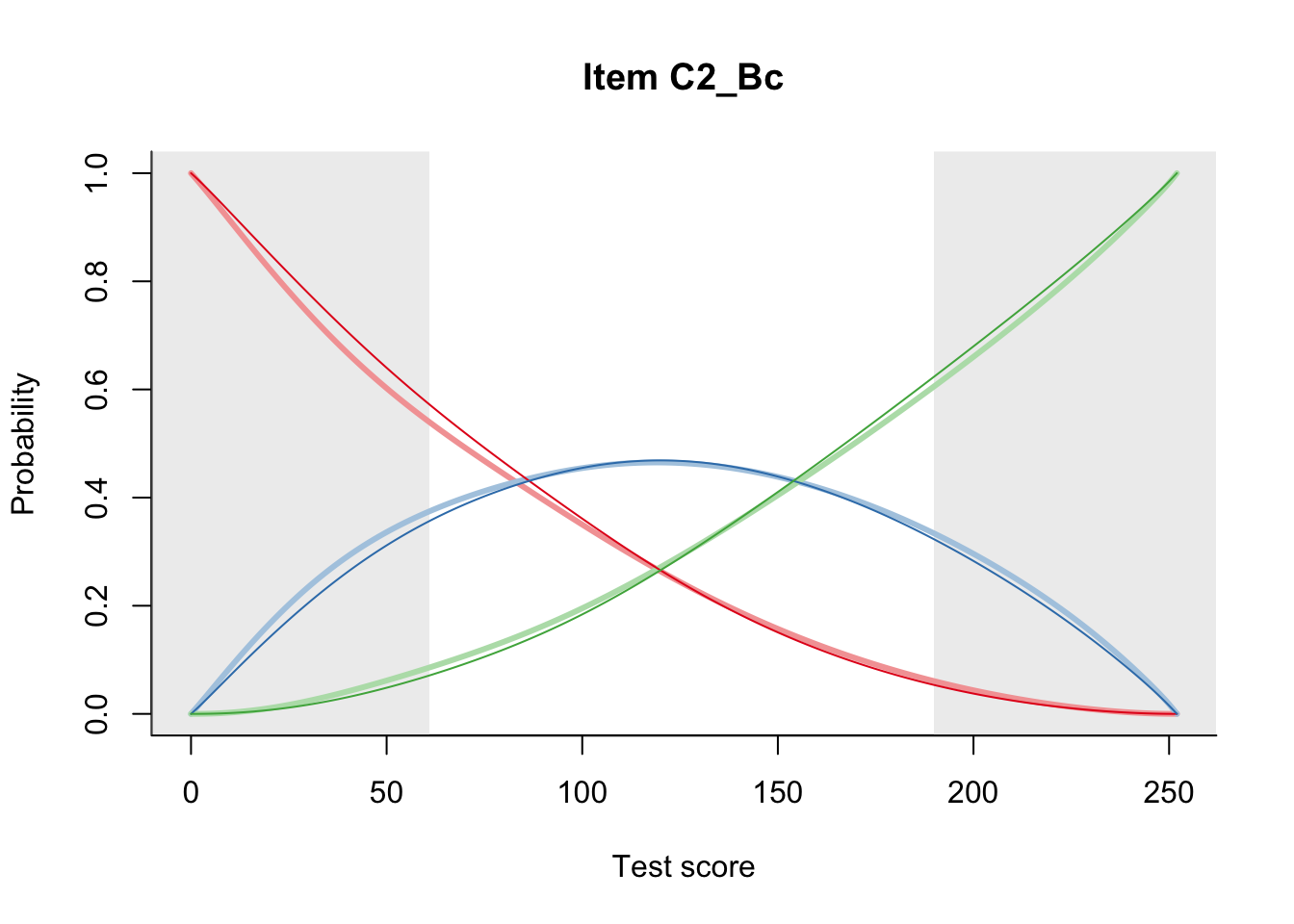
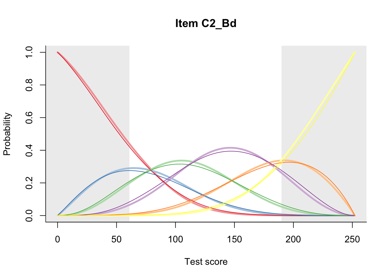
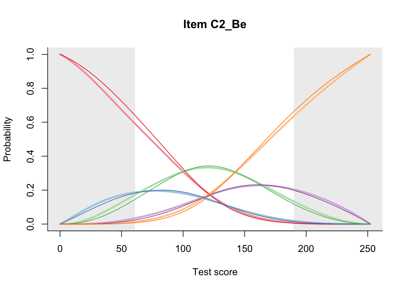
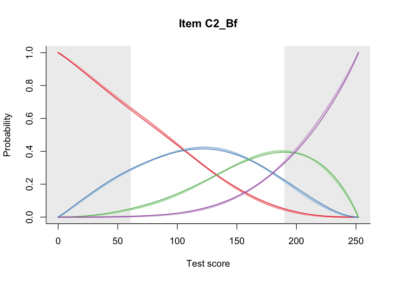
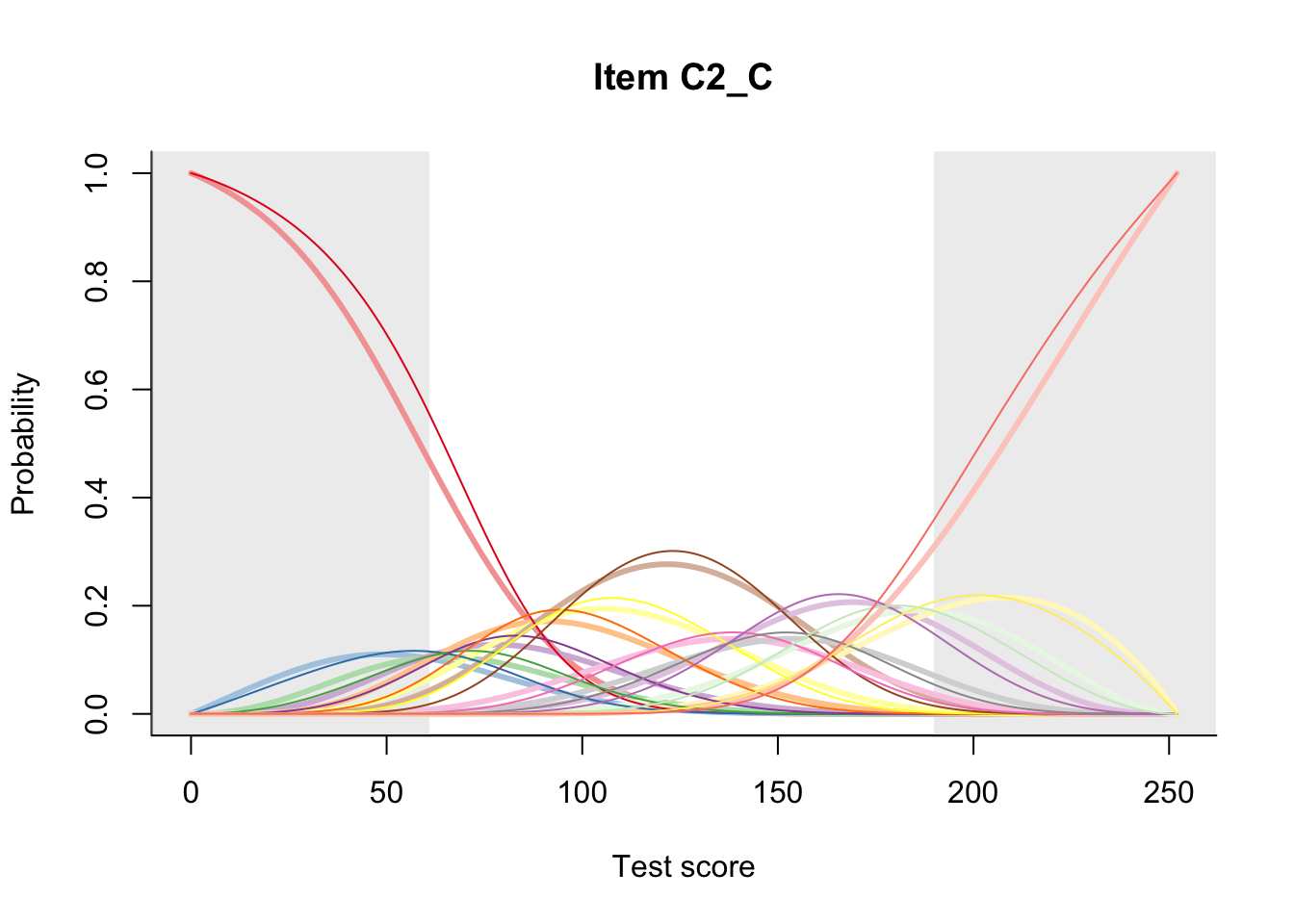
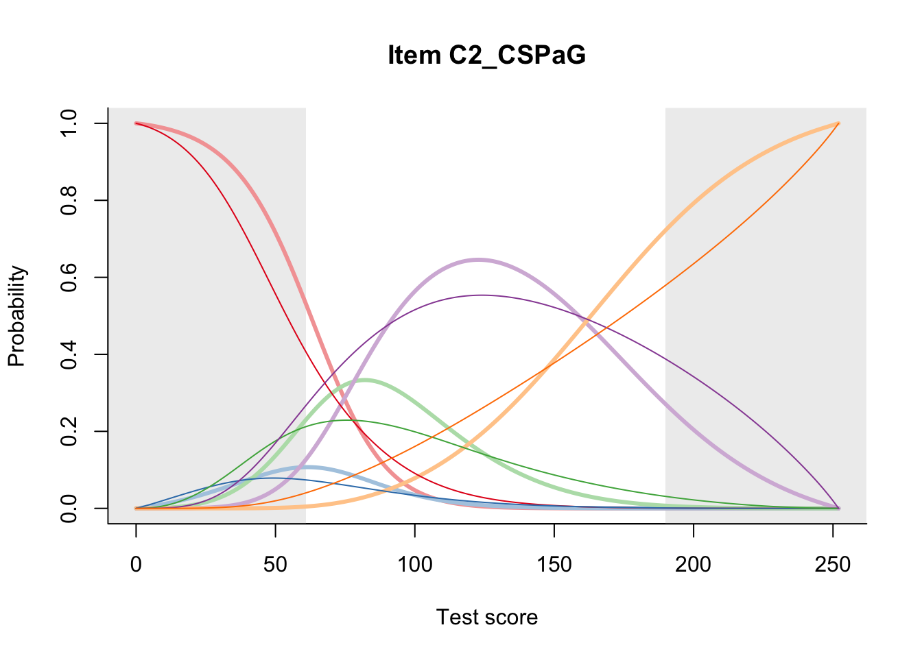
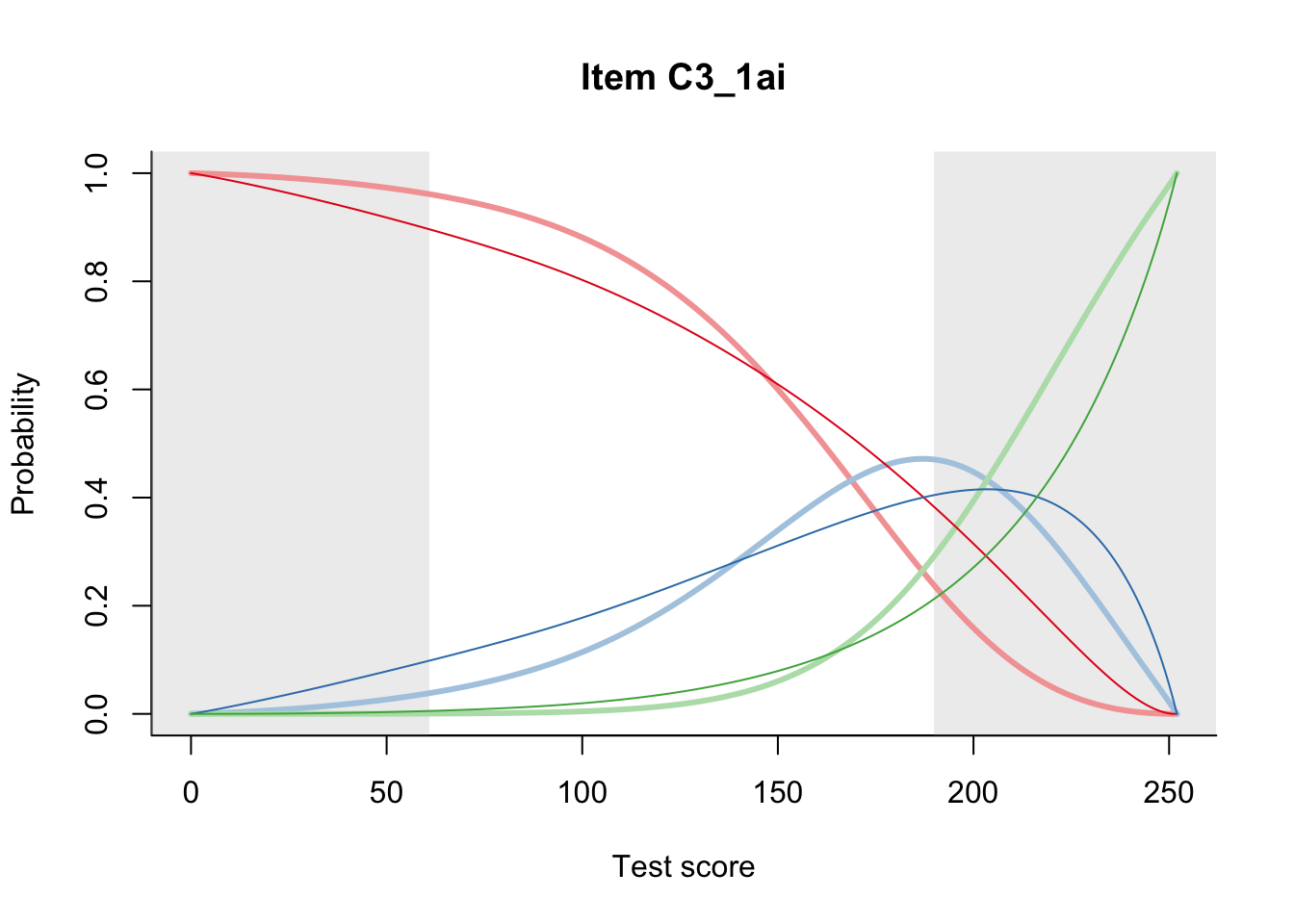
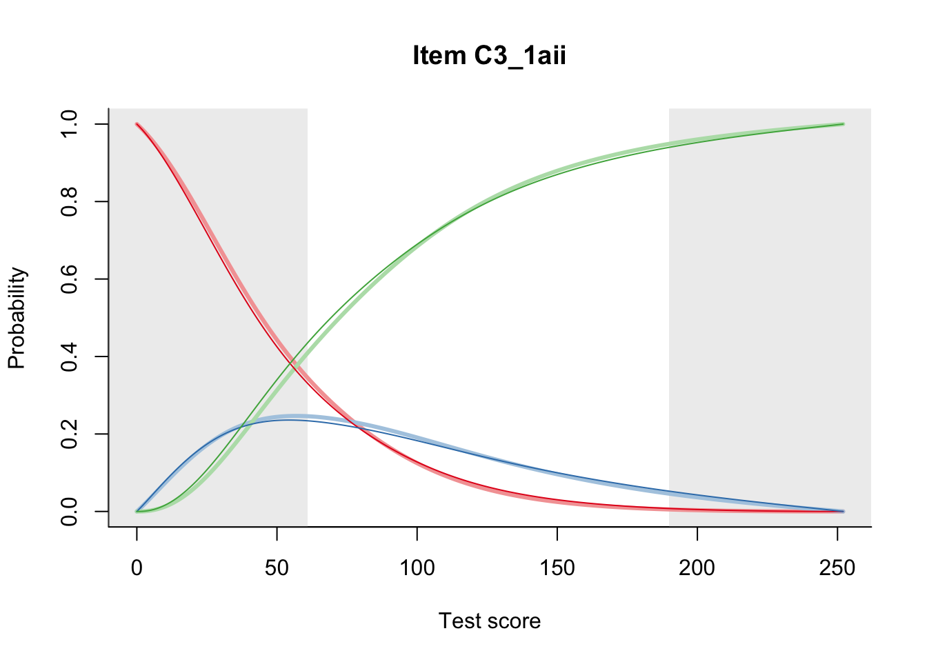
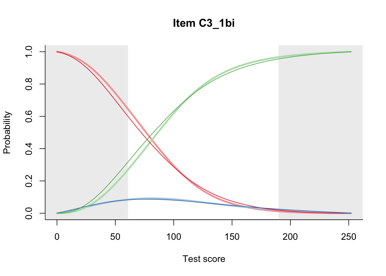
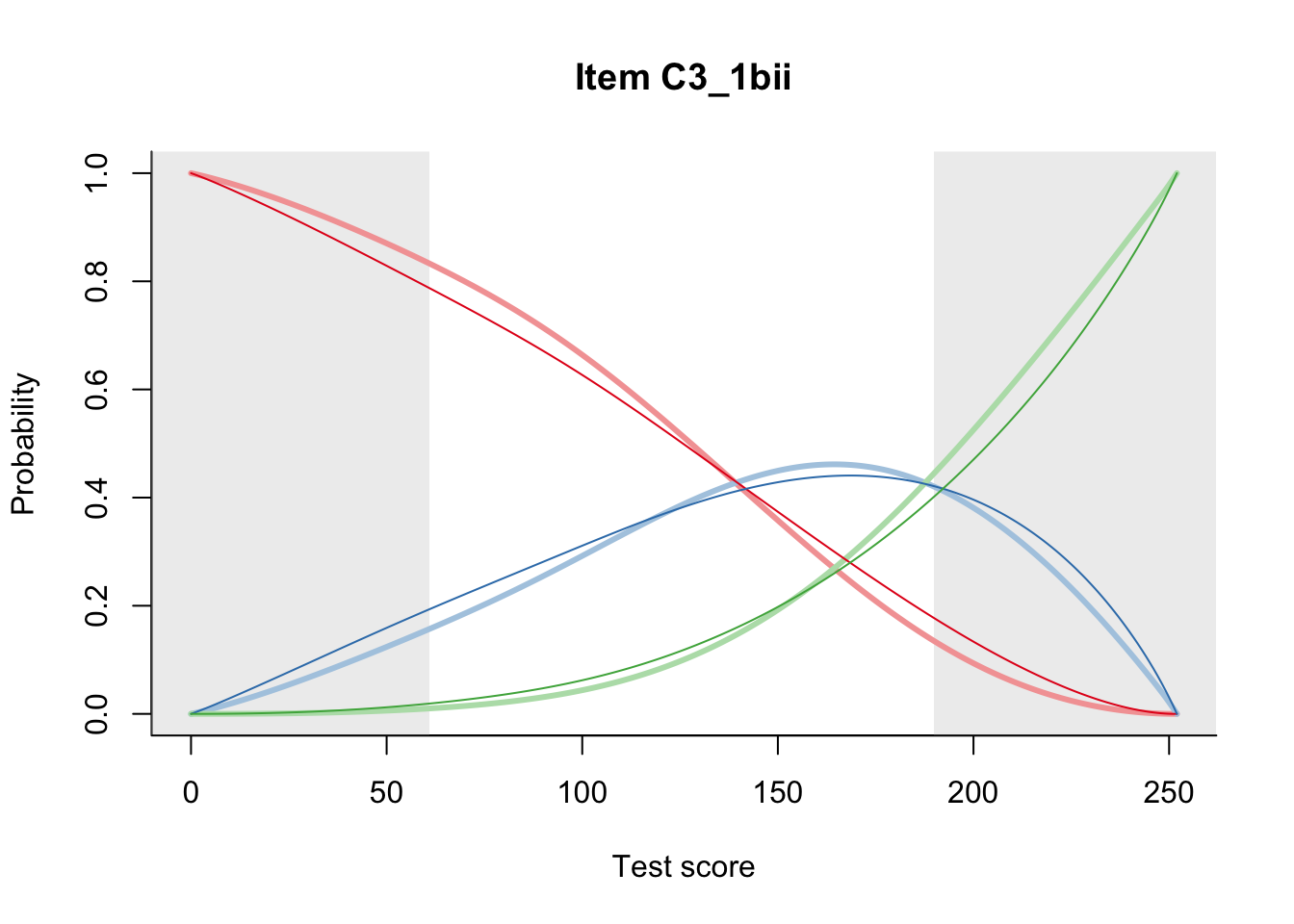
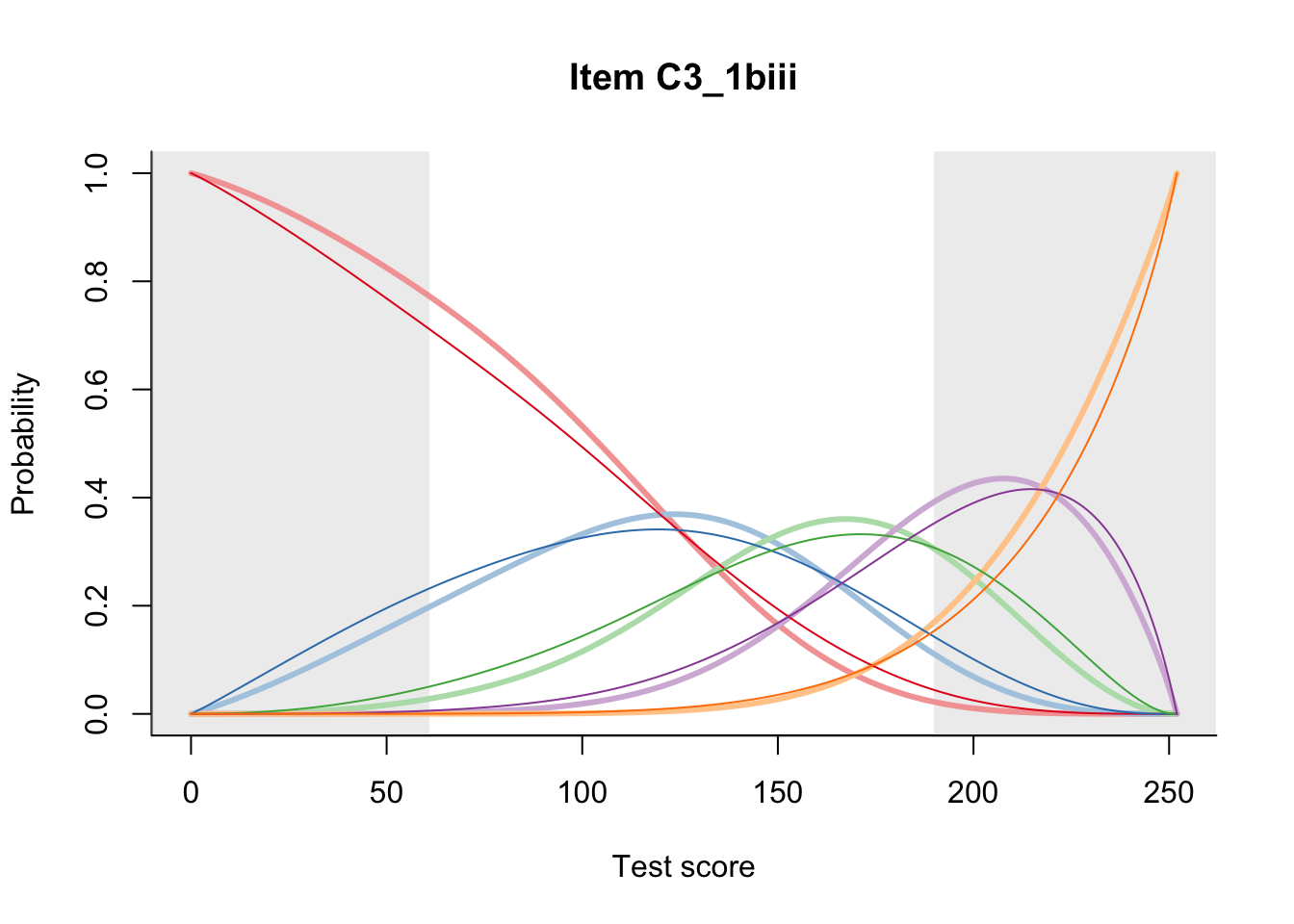
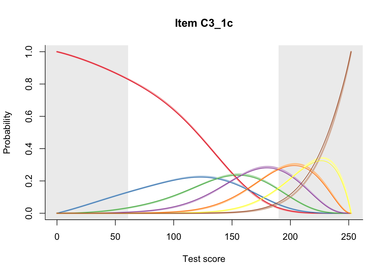
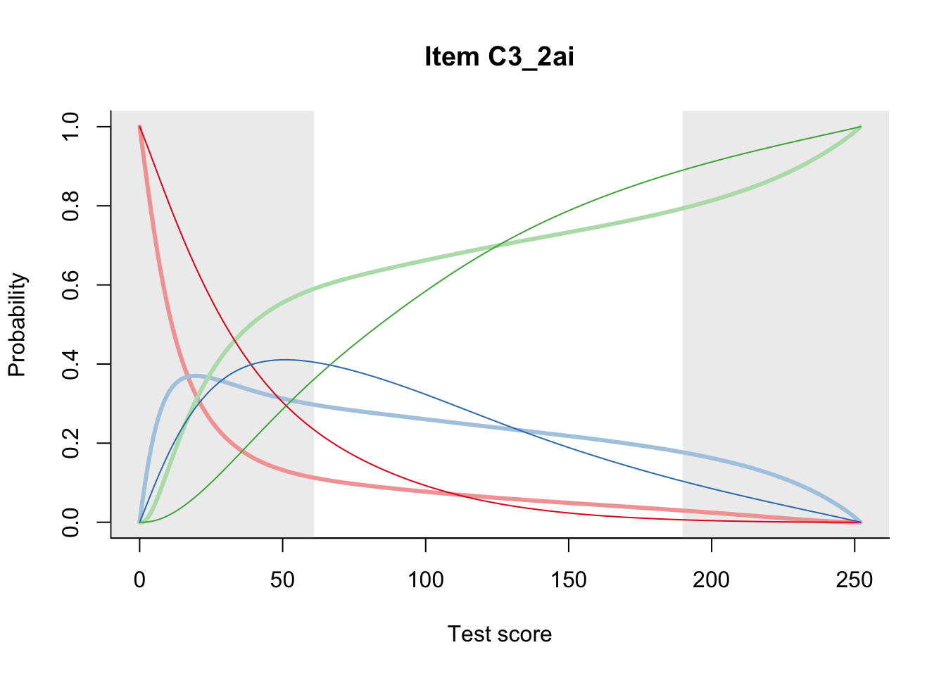
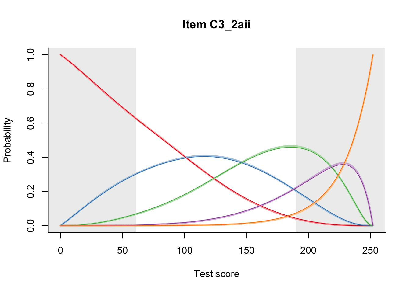
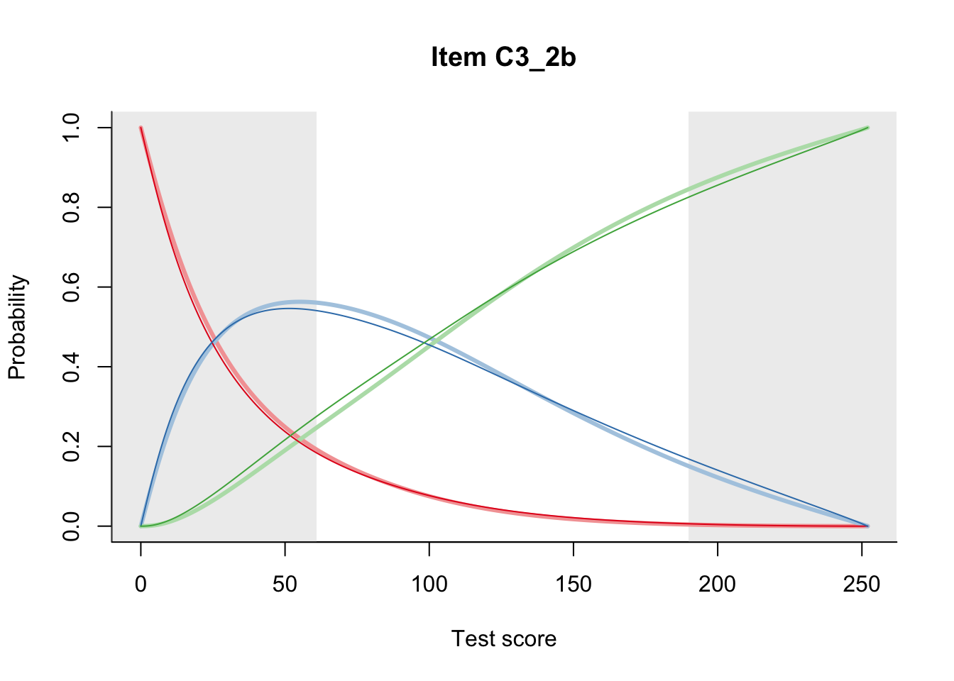
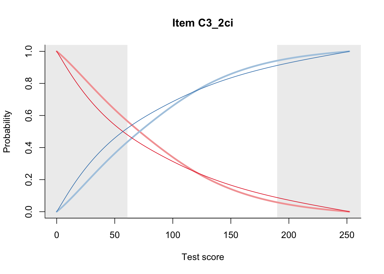
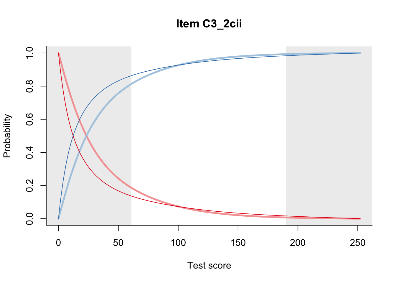
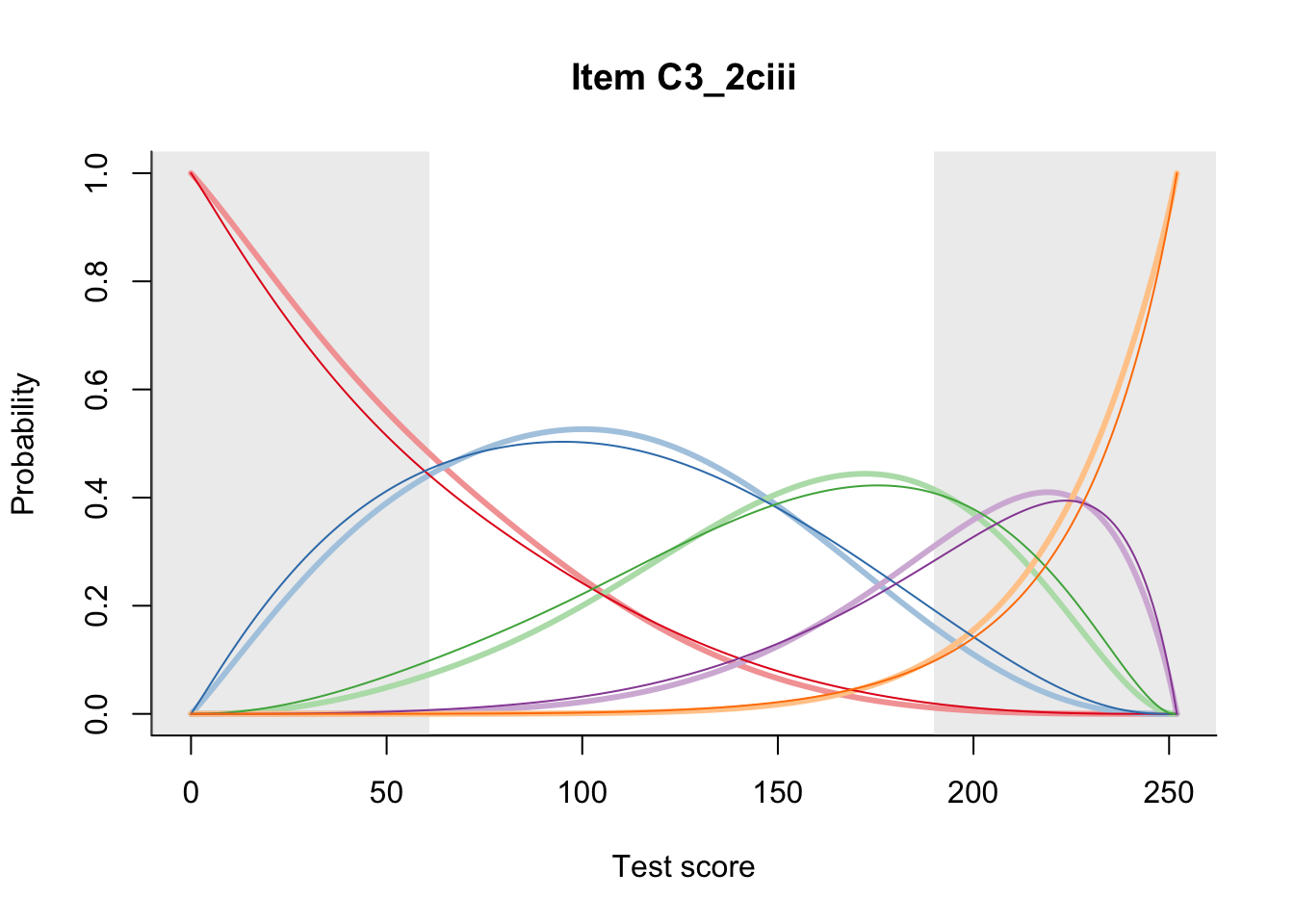
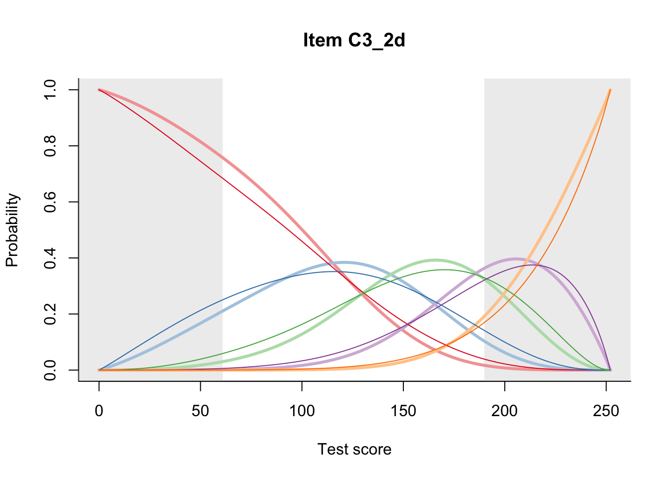
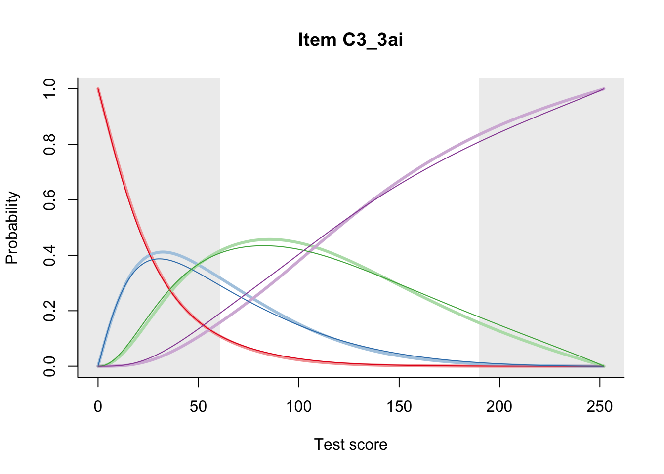
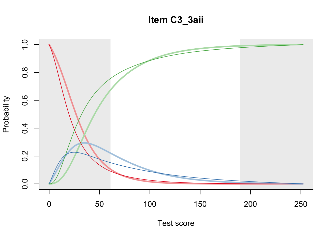
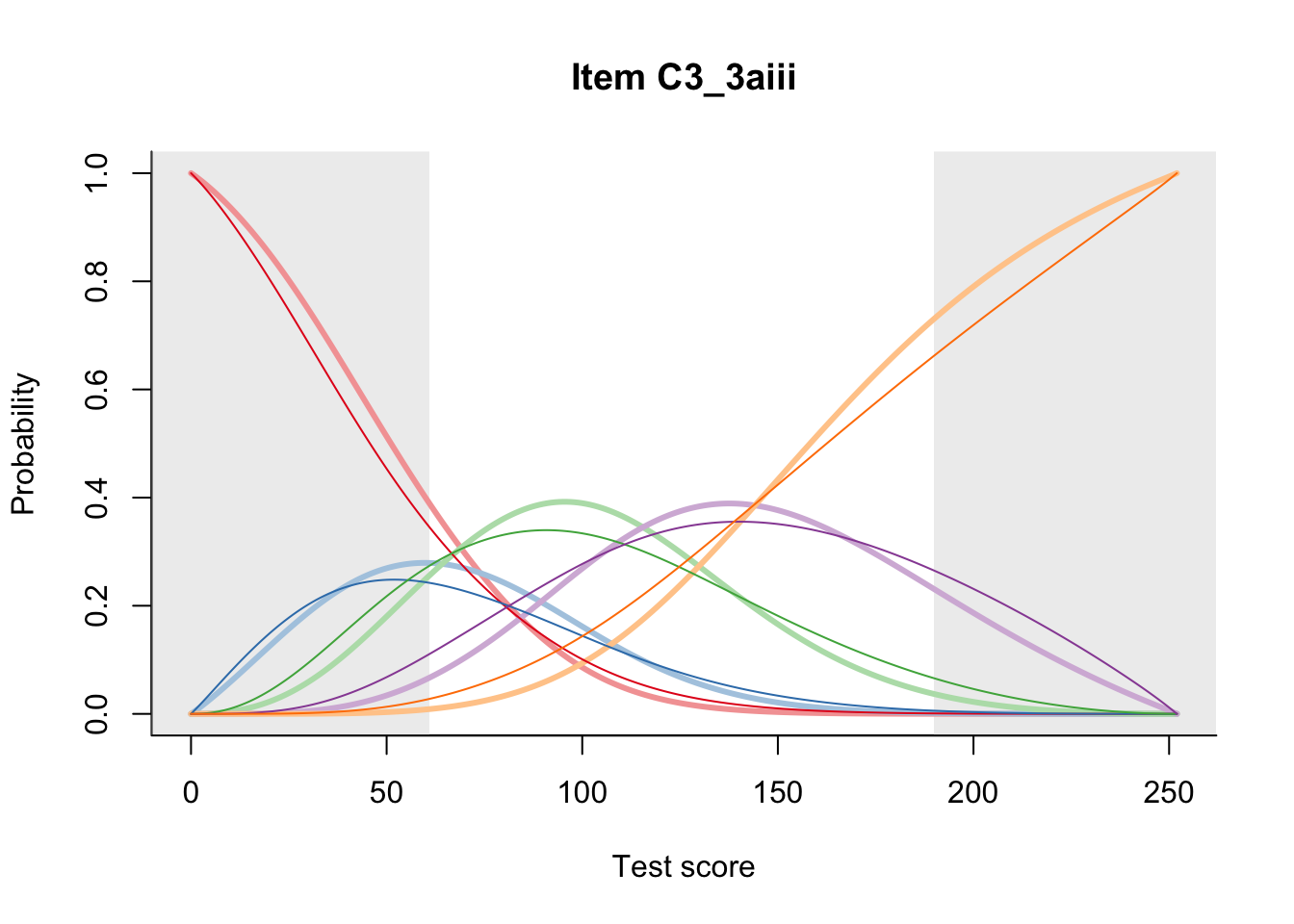
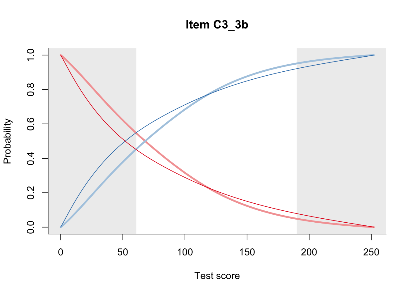
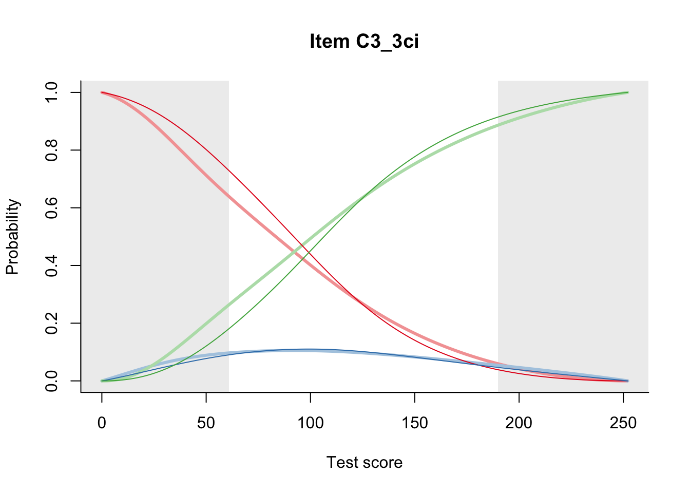
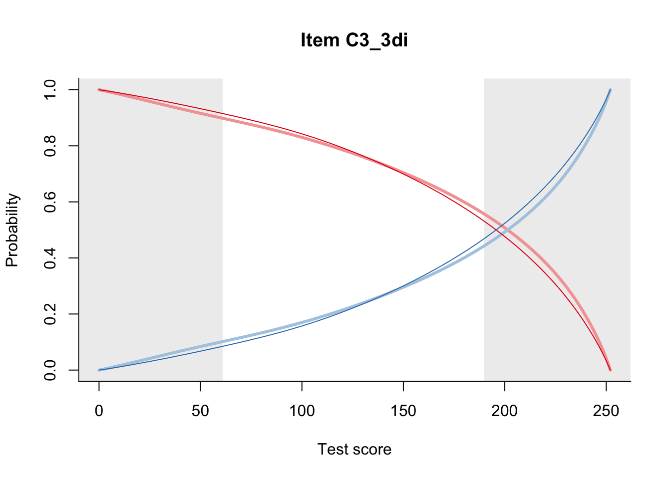
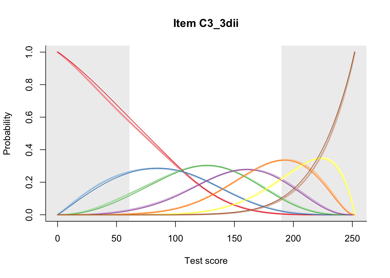
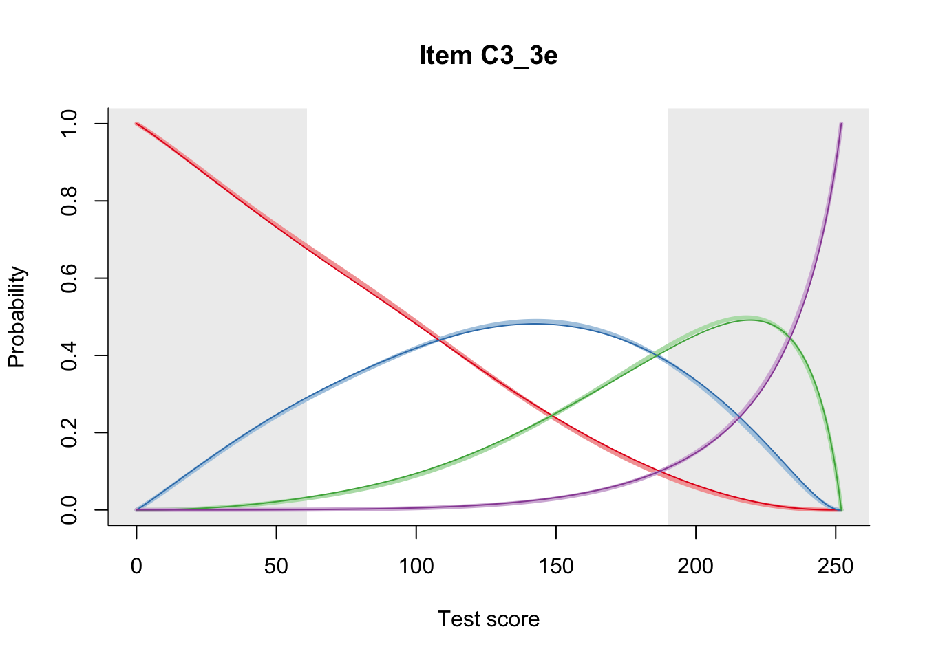
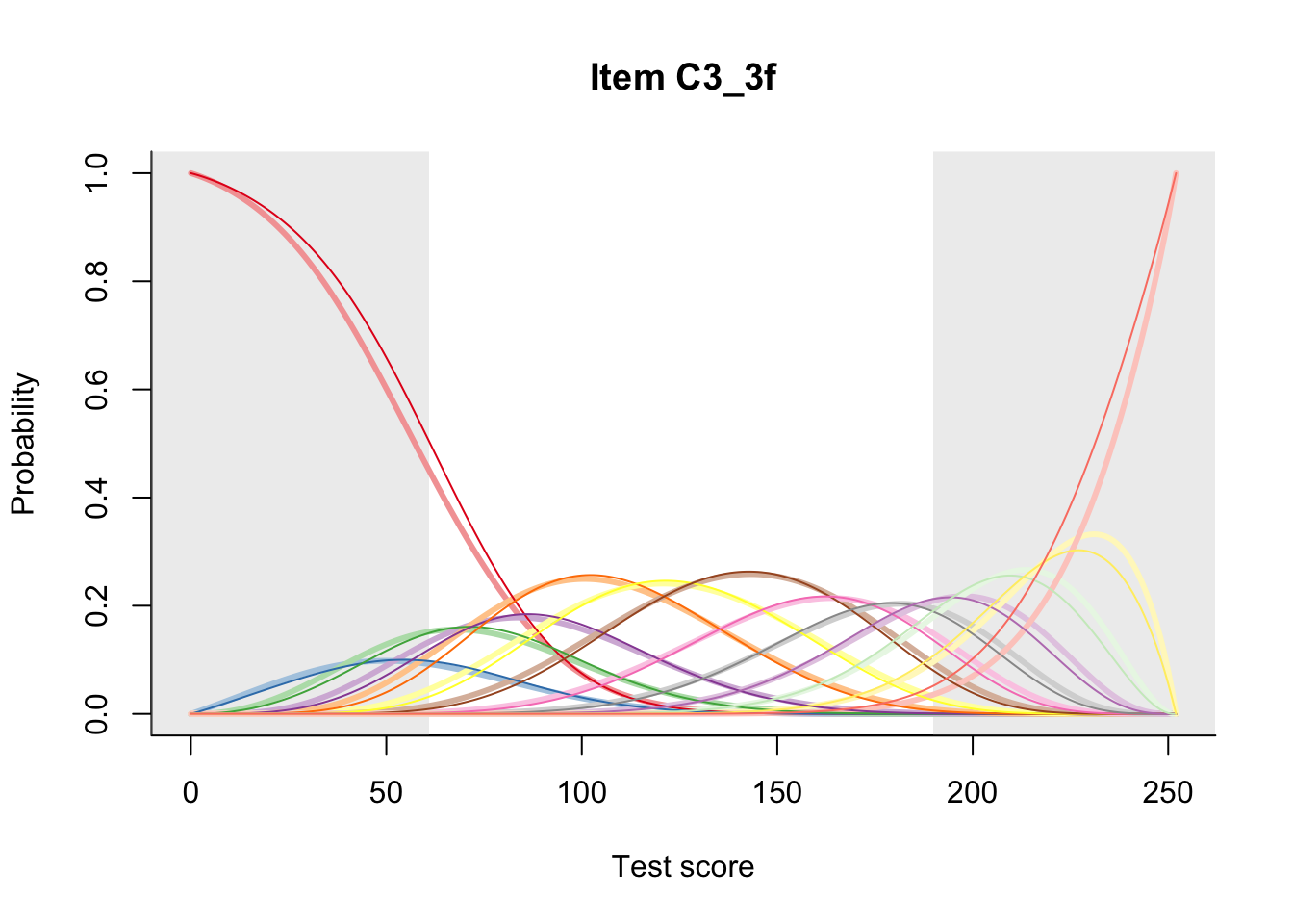
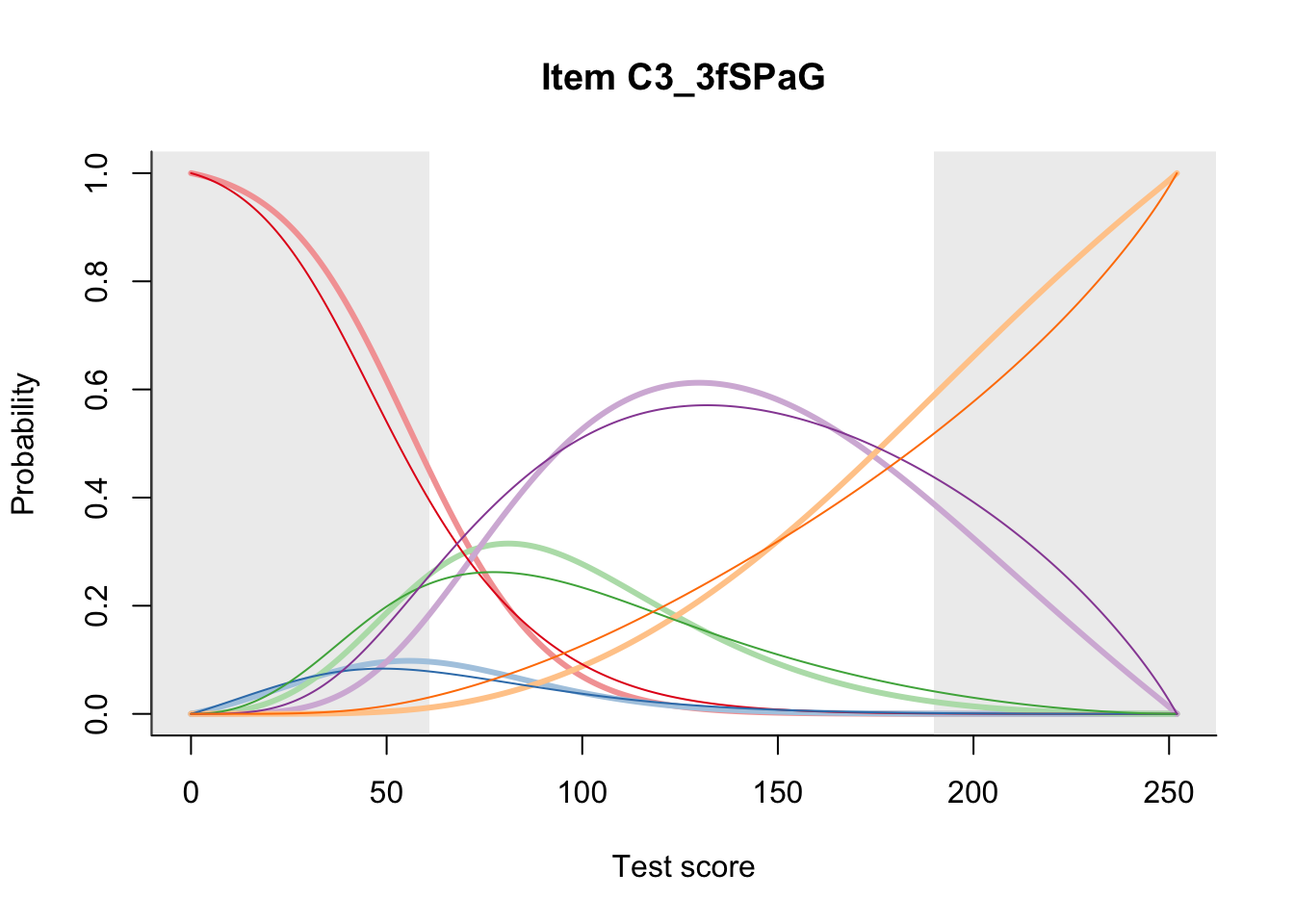
27.2 Item Difficulty

m = fit_inter(db)
n_items <- nrow(data_summary)
for(i in 1:n_items){
    plot(m, data_summary$Variable[i], summate=FALSE, show.observed=FALSE)
}

# plot(m, "C3_1ai", summate=FALSE, show.observed=FALSE)
# plot(m, "C3_1ai", summate=TRUE, show.observed=TRUE)

close_project(db)

27.3 Take a look at the SPAG items. How well are they working?

Andrich, David, and Ida Marais. 2019. “The Idea of Measurement.” In A Course in Rasch Measurement Theory, 3–11. Springer Nature Singapore. https://doi.org/10.1007/978-981-13-7496-8_1.

Bond, Trevor G., Zi Yan, and Moritz Heene. 2020. Applying the Rasch Model: Fundamental Measurement in the Human Sciences. Routledge. https://doi.org/10.4324/9780429030499.

Cappelleri, Jason Lundy, J. C. 2014. “Overview of Classical Test Theory and Item Response Theory for the Quantitative Assessment of Items in Developing Patient-Reported Outcomes Measures.” Clinical Therapeutics 36 (5): 648–62. https://doi.org/https://doi.org/10.1016/j.clinthera.2014.04.006.

Cronbach, Lee J. 1951. “Coefficient Alpha and the Internal Structure of Tests.” Psychometrika 16 (3): 297–334. https://doi.org/10.1007/bf02310555.

Goldstein, H., and Steve Blinkhorn. 1982. “The Rasch Model Still Does Not Fit.” British Educational Research Journal 8 (2): 167–70. https://doi.org/10.1080/0141192820080207.

Lord, Frederic M, and Melvin R Novick. 2008. Statistical Theories of Mental Test Scores. IAP.

McNeish, Daniel. 2018. “Thanks Coefficient Alpha, We’ll Take It from Here.” Psychological Methods 23 (3): 412–33. https://doi.org/10.1037/met0000144.

Panayides, Panayiotis, Colin Robinson, and Peter Tymms. 2010. “The Assessment Revolution That Has Passed England by: Rasch Measurement.” British Educational Research Journal 36 (4): 611–26. https://doi.org/10.1080/01411920903018182.

Robitzsch, Alexander, Thomas Kiefer, and Margaret Wu. 2022. TAM: Test Analysis Modules. https://CRAN.R-project.org/package=TAM.

Sijtsma, Klaas. 2008. “On the Use, the Misuse, and the Very Limited Usefulness of Cronbach’s Alpha.” Psychometrika 74 (1): 107–20. https://doi.org/10.1007/s11336-008-9101-0.

Wright, Benjamin D, and Magdalena Mok. 2000. “Rasch Models Overview.” Journal of Applied Measurement 1 (1): 83–106.