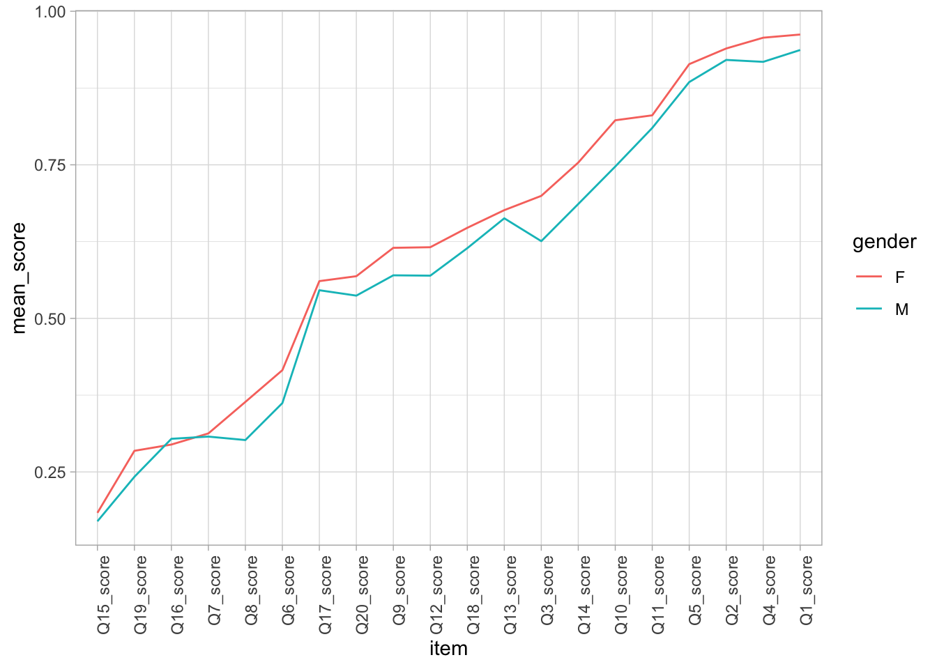
13.6 Plot the ordered responses as a line graph, grouped by gender with item on the x-axis, mean_score on the y-axis
p <-ggplot(ordered_responses, aes(x=item, y=mean_score, group=gender, colour=gender, line_style=gender))p <- p +geom_line() # rotate the x-axis labelsp <- p +theme_light()p <- p +theme(axis.text.x =element_text(angle =90, hjust =1))p
Andrich, David, and Ida Marais. 2019. “The Idea of Measurement.” In A Course in Rasch Measurement Theory, 3–11. Springer Nature Singapore. https://doi.org/10.1007/978-981-13-7496-8_1.
Bond, Trevor G., Zi Yan, and Moritz Heene. 2020. Applying the Rasch Model: Fundamental Measurement in the Human Sciences. Routledge. https://doi.org/10.4324/9780429030499.
Cappelleri, Jason Lundy, J. C. 2014. “Overview of Classical Test Theory and Item Response Theory for the Quantitative Assessment of Items in Developing Patient-Reported Outcomes Measures.”Clinical Therapeutics 36 (5): 648–62. https://doi.org/https://doi.org/10.1016/j.clinthera.2014.04.006.
Cronbach, Lee J. 1951. “Coefficient Alpha and the Internal Structure of Tests.”Psychometrika 16 (3): 297–334. https://doi.org/10.1007/bf02310555.
Goldstein, H., and Steve Blinkhorn. 1982. “The Rasch Model Still Does Not Fit.”British Educational Research Journal 8 (2): 167–70. https://doi.org/10.1080/0141192820080207.
Lord, Frederic M, and Melvin R Novick. 2008. Statistical Theories of Mental Test Scores. IAP.
McNeish, Daniel. 2018. “Thanks Coefficient Alpha, We’ll Take It from Here.”Psychological Methods 23 (3): 412–33. https://doi.org/10.1037/met0000144.
Panayides, Panayiotis, Colin Robinson, and Peter Tymms. 2010. “The Assessment Revolution That Has Passed England by: Rasch Measurement.”British Educational Research Journal 36 (4): 611–26. https://doi.org/10.1080/01411920903018182.
Sijtsma, Klaas. 2008. “On the Use, the Misuse, and the Very Limited Usefulness of Cronbach’s Alpha.”Psychometrika 74 (1): 107–20. https://doi.org/10.1007/s11336-008-9101-0.
Wright, Benjamin D, and Magdalena Mok. 2000. “Rasch Models Overview.”Journal of Applied Measurement 1 (1): 83–106.