rm(list=ls())
library(tidyverse)
library(ggplot2)
library(sirt)
require(nmmBtm)
library(ggrepel)
decisions_1 <- read_csv('data/decisions-1.csv')
persons_1 <- read_csv('data/persons-1.csv')
decisions_2 <- read_csv('data/decisions-2.csv')
persons_2 <- read_csv('data/persons-2.csv')31 Linking & Equating
Whenever you calibrate a Rasch model or a CJ model the scale you use is arbitrary. That means that you cannot compare two separate CJ or Rasch calibrations as the scales they use will be different. To place two calibrations on the same scale you need to link them with common items.
To illustrate this point, the dataset decisions-2 has the decisions from a CJ session with the numbers 3 to 8. Fit the Bradley-Terry model to decisions-1 and decisions-2.
fit_btm_model <- function(persons, decisions, anchors=NULL){

    # get the person ids and their first names
    persons <- persons %>%
    select(Code, `First Name`) %>%
    rename(id = Code, name = `First Name`)

    # go through the decisions and add a column with the name of the person who was chosen or not chosen in each case
    decisions <- decisions %>% left_join(persons, by = c('chosen' = 'id')) %>%
    rename(chosenName = name) %>%
    left_join(persons, by = c('notChosen' = 'id')) %>%
    rename(notChosenName = name)

    # mutate chosenName and notChosenName to be factors
    decisions <- decisions %>%
    mutate(chosenName = factor(chosenName), notChosenName = factor(notChosenName))

    # format for the btm model
    decisions <- decisions %>%
    select(chosenName, notChosenName) %>%
    mutate(result = 1)

    # the package doesn't like tibbles?
    decisions <- as.data.frame(decisions)
    mod1 <- btm(decisions, fix.theta = anchors, fix.eta = 0, ignore.ties = TRUE, eps = 0.3)
    return (mod1)

}

mdl1 <- fit_btm_model(persons_1, decisions_1)
mdl2 <- fit_btm_model(persons_2, decisions_2)
31.1 Comparing the model effects
Plot the relationship between the model effects for decisions-1 against decisions-2. What do you notice?
# get the model effects for the two models
effects_1 <- mdl1$effects
effects_2 <- mdl2$effects
combined_effects <- effects_1 %>% left_join(effects_2, by = c('individual'))

# plot the model effects.x against model effects.y
p <- combined_effects %>%
    ggplot(aes(x = theta.x, y = theta.y, label=individual)) +
    geom_point() +
    geom_text_repel() +
    geom_abline(intercept = 0, slope = 1, color = 'red') +
    labs(x = 'Model effects for decisions-1', y = 'Model effects for decisions-2') +
    theme_bw()
print(p)
Warning: Removed 2 rows containing missing values or values outside the scale range
(`geom_point()`).Warning: Removed 2 rows containing missing values or values outside the scale range
(`geom_text_repel()`).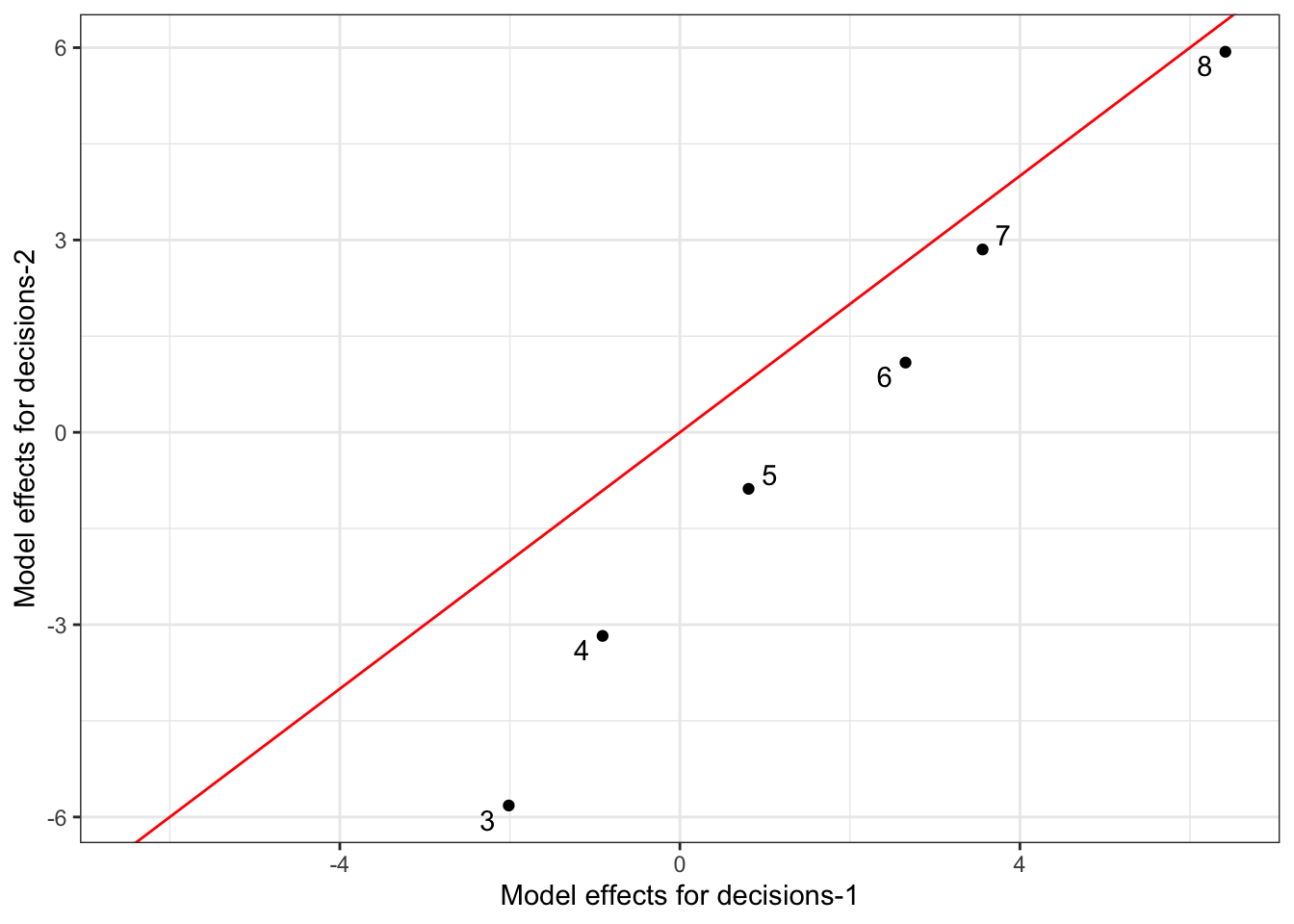
31.2 How do we place the two models on the same scale?
We can fix some of the item parameters between the calibrations.
# fix the item parameters for numbers 3, 5 & 7
anchors <- c(-2.0130565,0.8080052,3.5605796)
names(anchors) <- c('3','5','7')

mdl3 <- fit_btm_model(persons_2, decisions_2, anchors)
31.3 Now compare the model effects between model 1 and model 3
effects_3 <- mdl3$effects
combined_effects <- effects_1 %>% left_join(effects_3, by = c('individual'))

# plot the model effects.x against model effects.y
p <- combined_effects %>%
    ggplot(aes(x = theta.x, y = theta.y, label=individual)) +
    geom_point() +
    geom_text_repel() +
    geom_abline(intercept = 0, slope = 1, color = 'red') +
    labs(x = 'Model effects for  model 1', y = 'Model effects for model 2') +
    theme_bw()
print(p)
Warning: Removed 2 rows containing missing values or values outside the scale range
(`geom_point()`).Warning: Removed 2 rows containing missing values or values outside the scale range
(`geom_text_repel()`).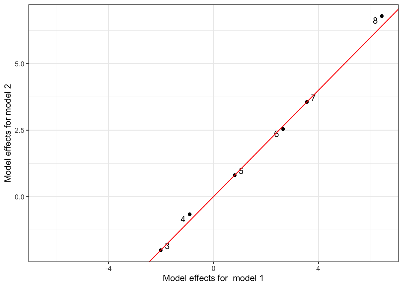
31.4 With the scales on the same scale we can now build scales across time & space
31.5 Extension exercise
Try different equating designs for different sets of numbers. eg. Try equating 1 to 8 with 6 to 13. How well does it work?