rm(list=ls())
library(tidyverse)
library(dexter)
# load in the dataset
responses <- read_csv('data/responses.csv')
keys <- read_csv('data/key.csv')
# Create the rules
rules <- keys_to_rules(keys, include_NA_rule = TRUE)
db <- start_new_project(rules, db_name = ":memory:", person_properties=list(gender="unknown"))17 Assessing the fit of the Rasch model
17.1 How does Rasch differ from regression models?
A common question is how does the Rasch model differ from regression models. The following article explains it well: https://dexter-psychometrics.github.io/dexter/articles/blog/2018-02-25-item-total-regressions-in-dexter. Read through the first three paragraphs and note the key difference.
17.2 Model predictions compared to the empirical data
If model predictions are reasonably similar to the empirical data then we can be relatively sure the model fits. While there are tests of ‘fit’ these statistical tests are of little use in evaluating the ways in which a test may fail to fit a model, and tend to be largely dependent on sample size. The dexter approach is built around visual inspections of Item Characteristic Plots. Note that dexter uses a slightly different model to the Rasch model for dichotomous data where there is no missing data.
17.3 Item Characteristic Plots
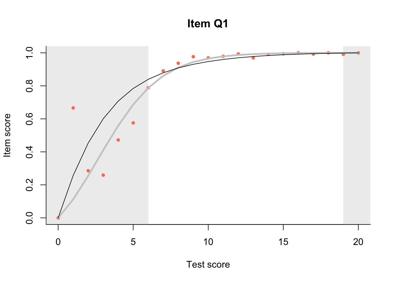
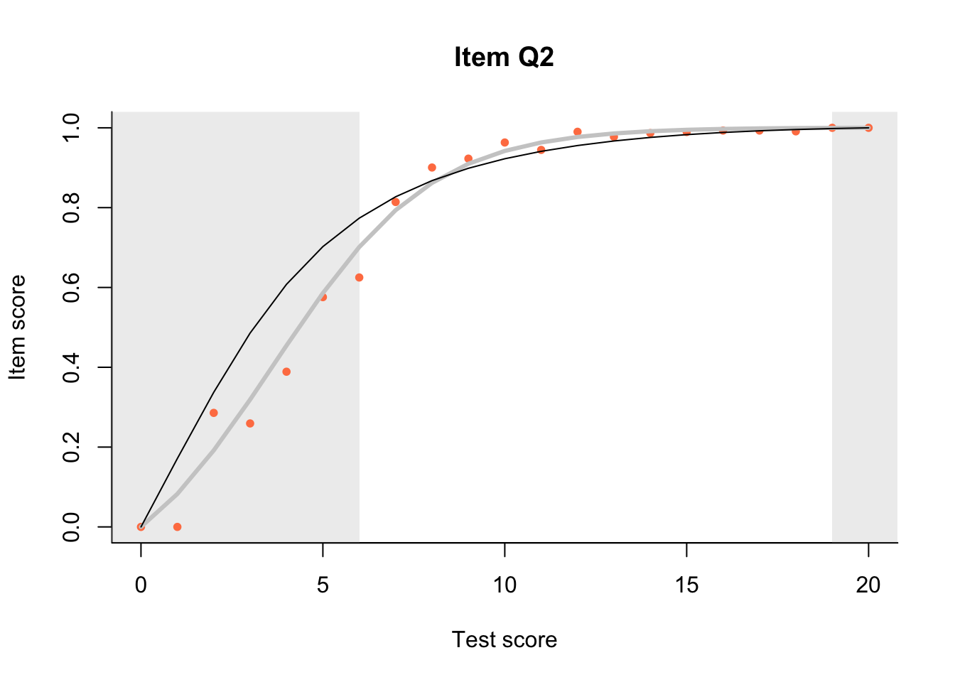
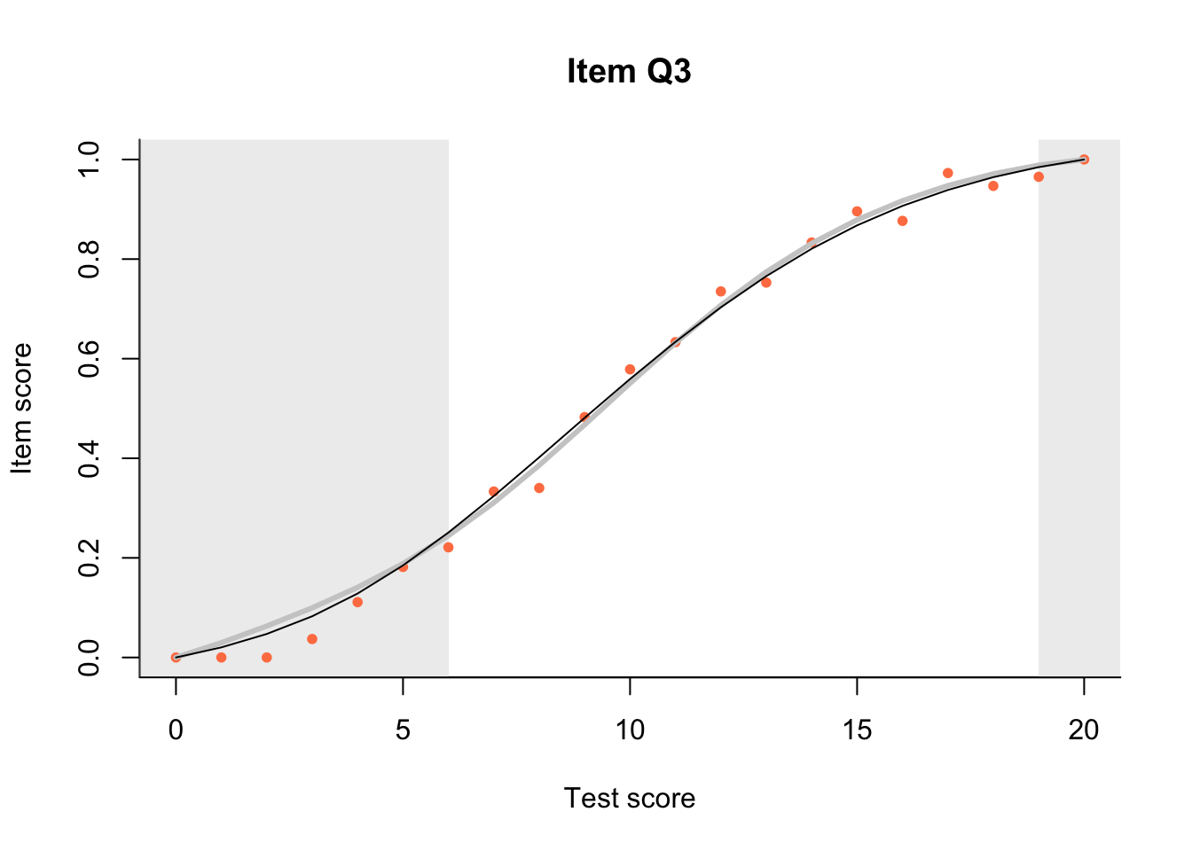
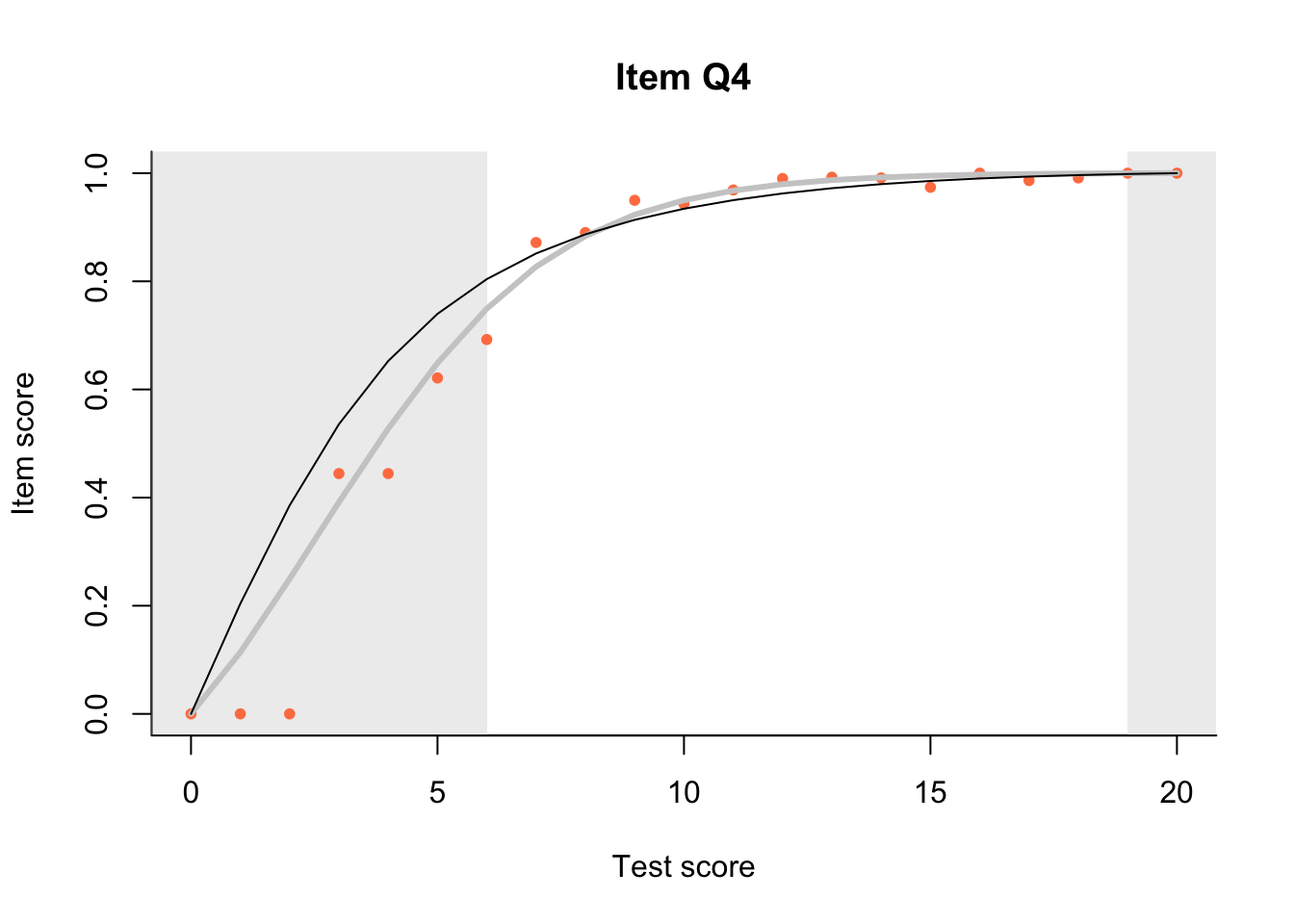
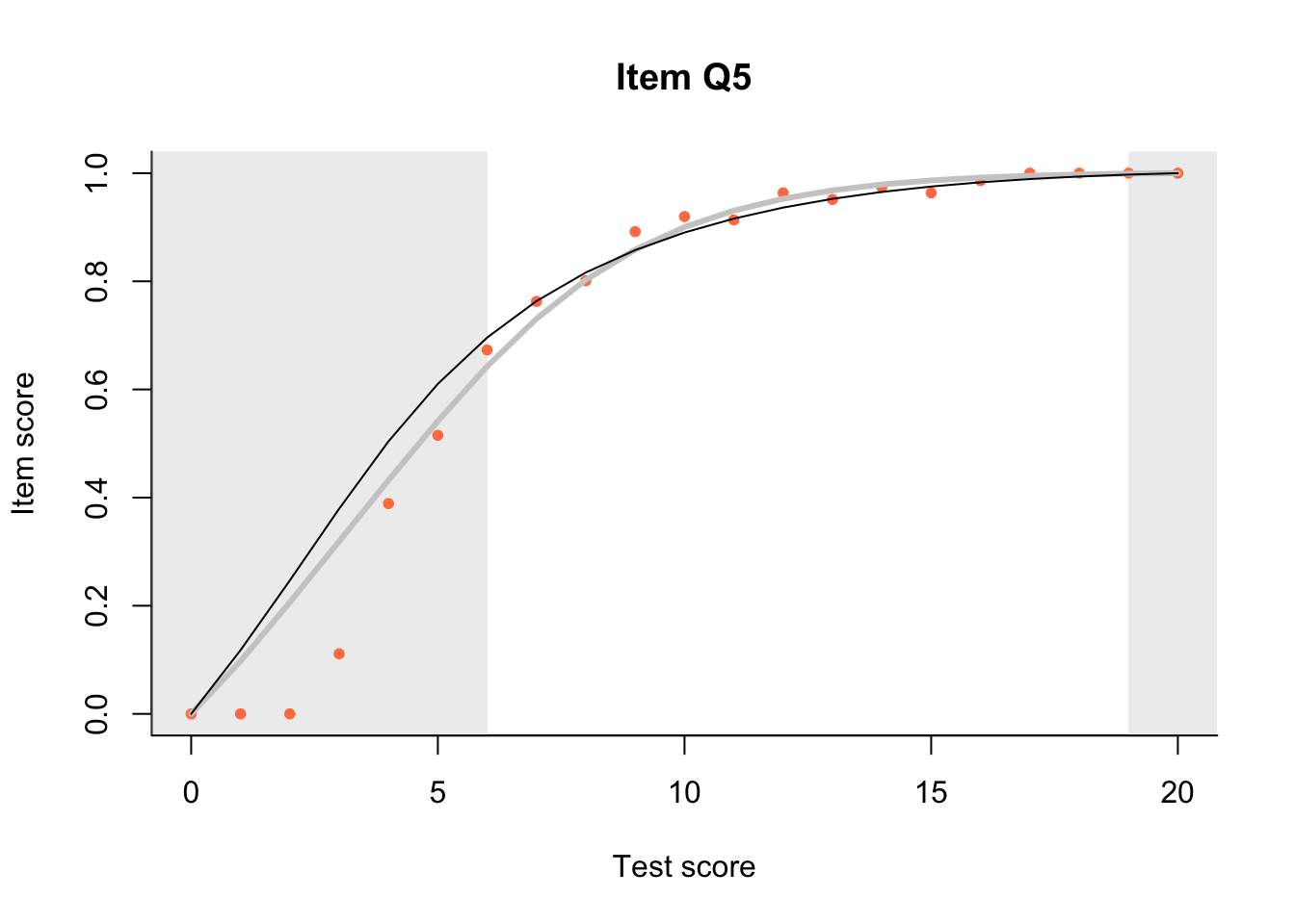
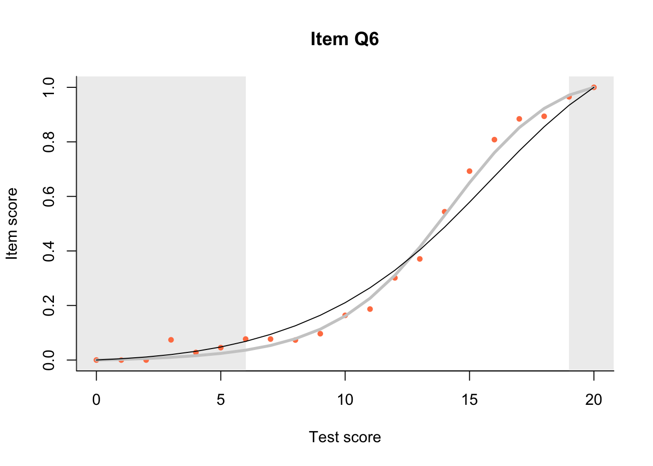
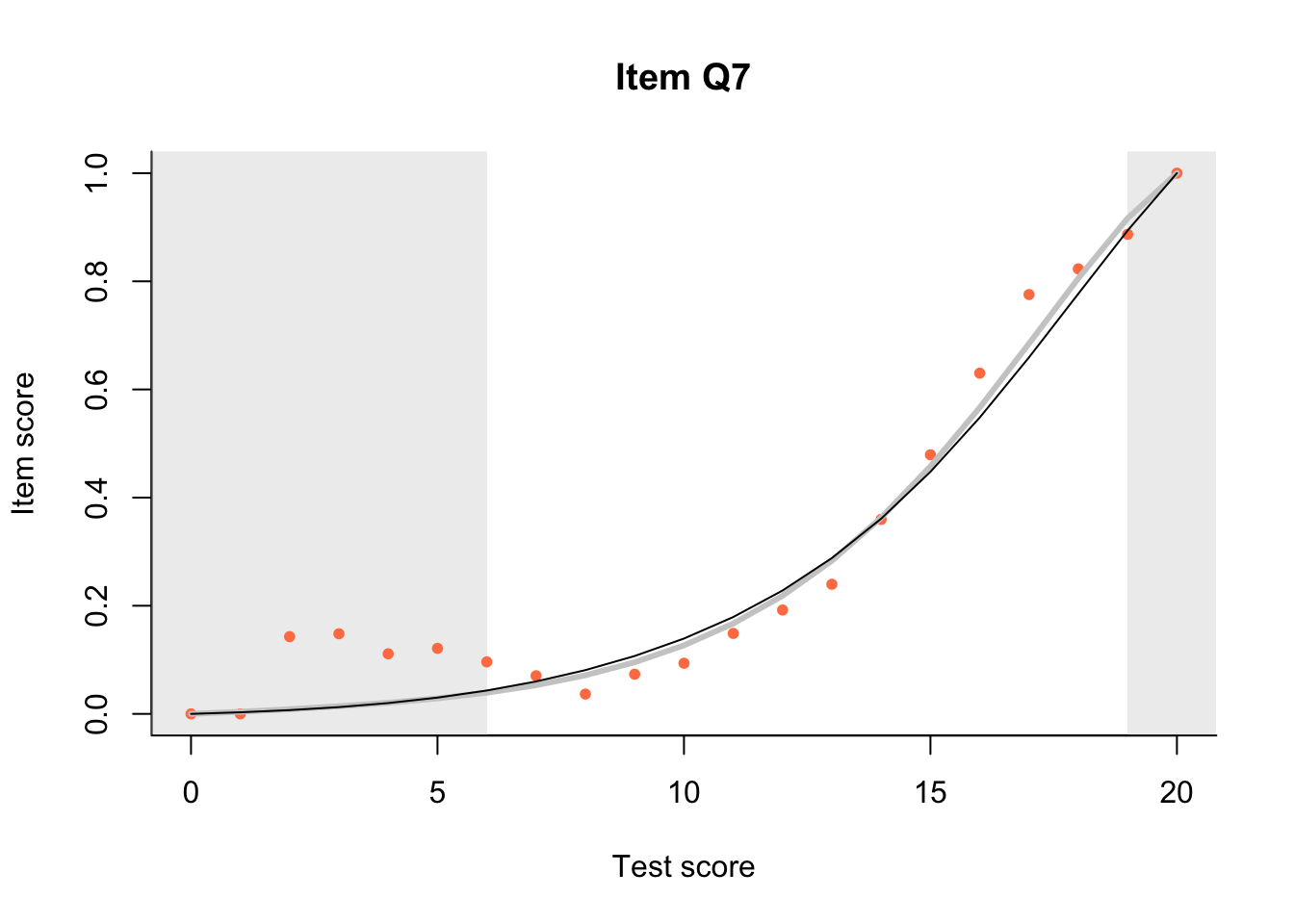
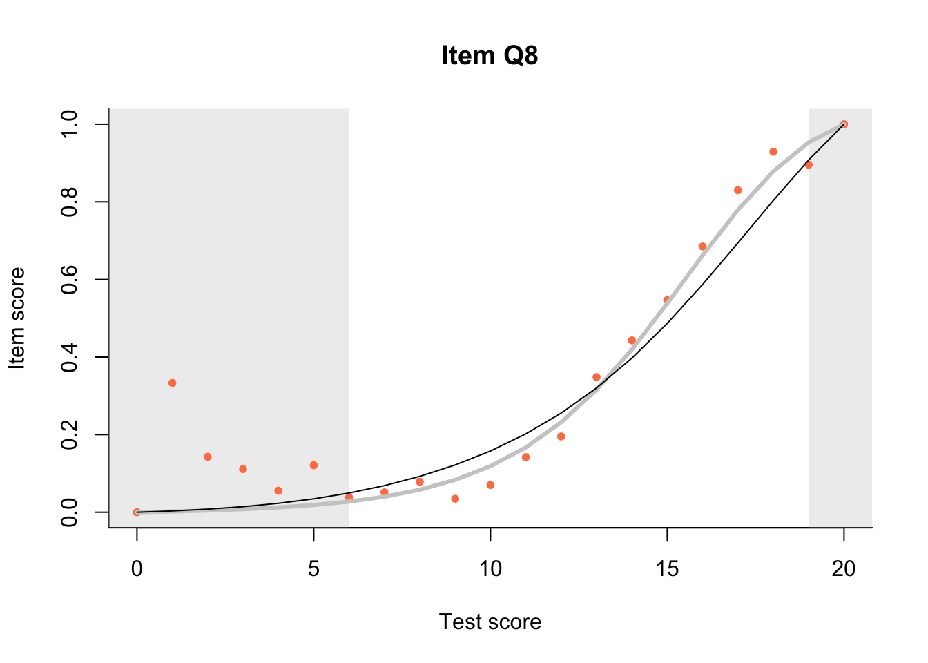
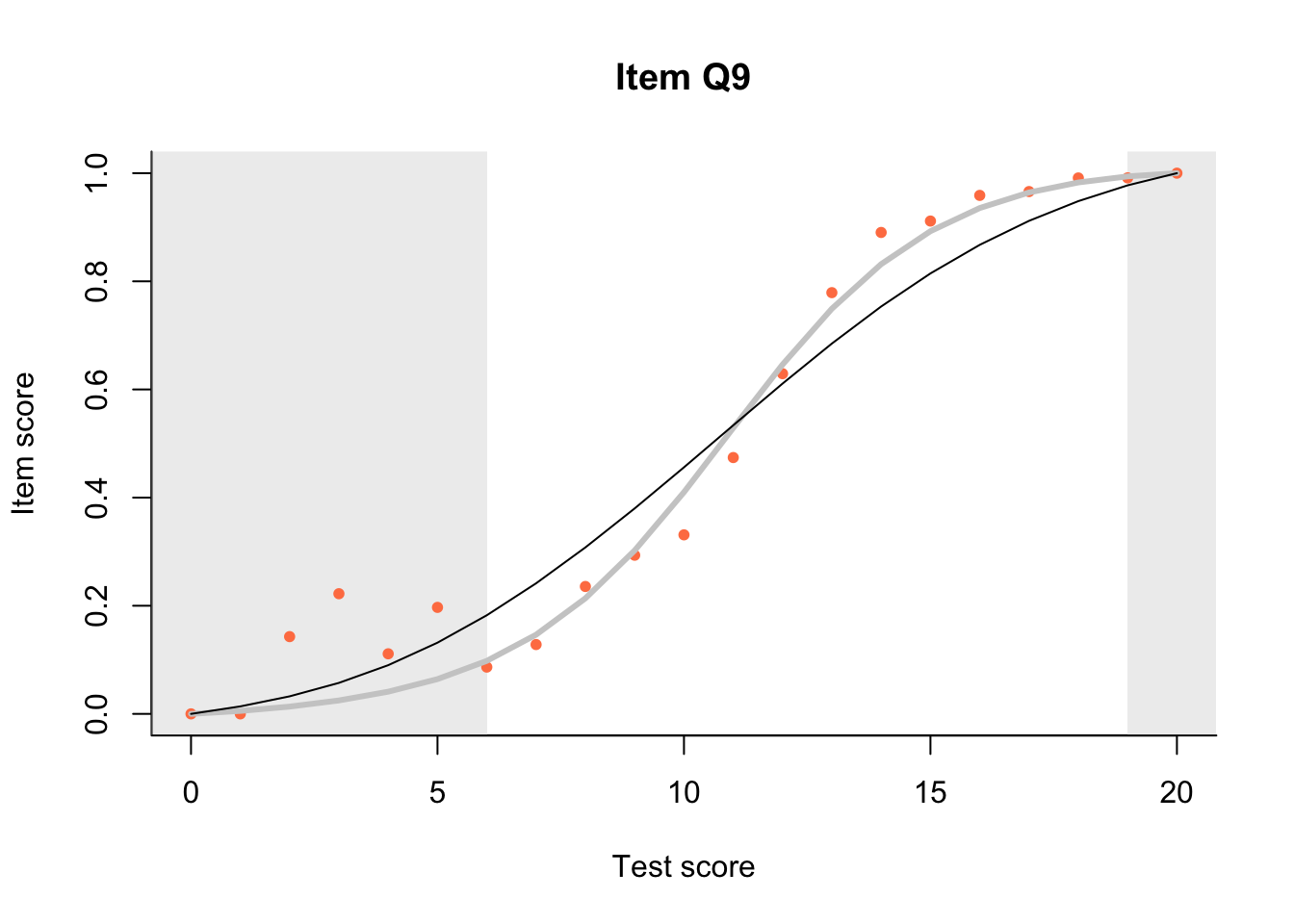
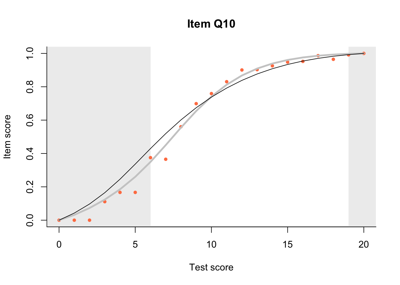
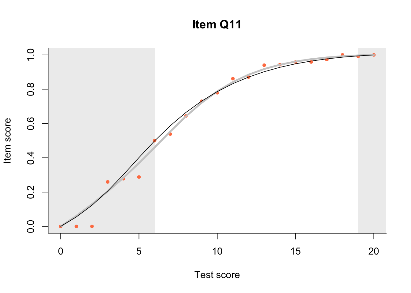
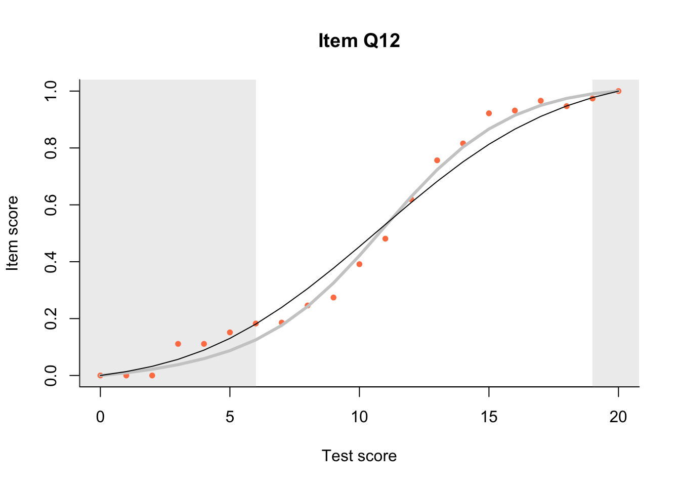
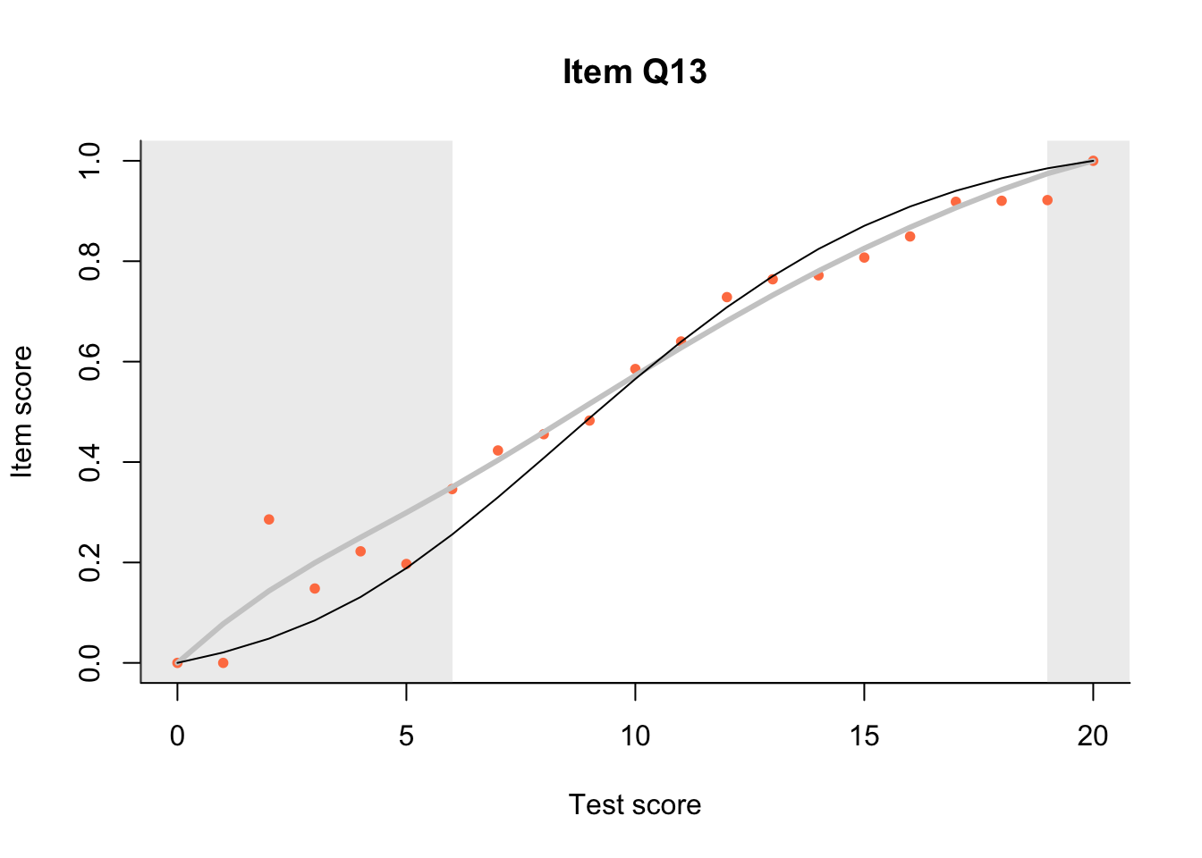
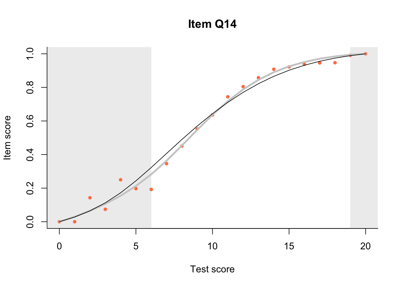
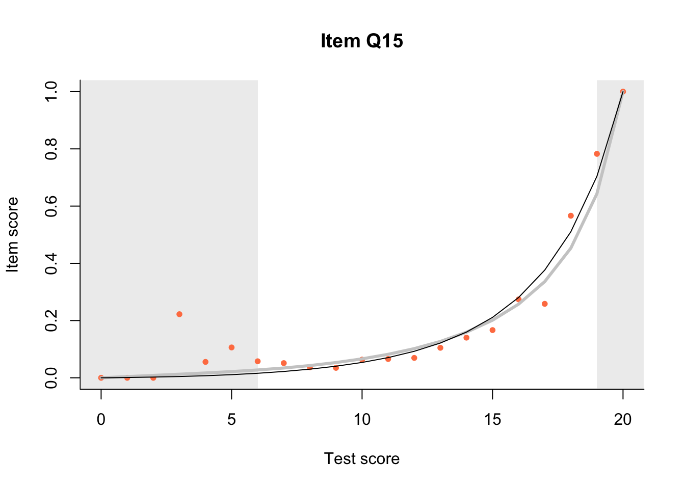
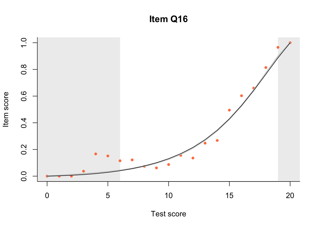
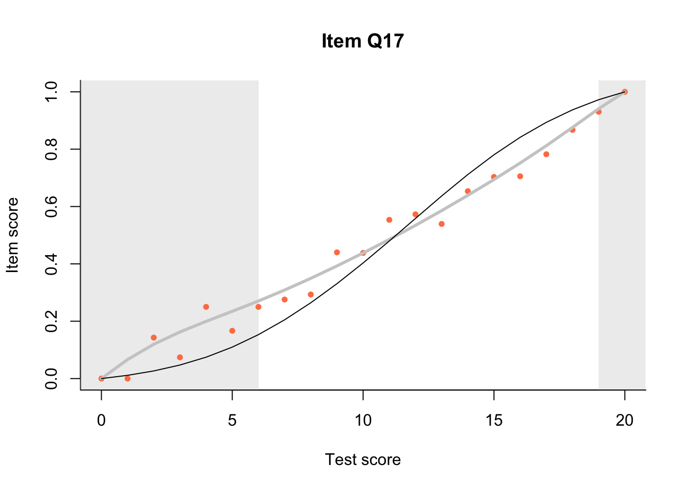
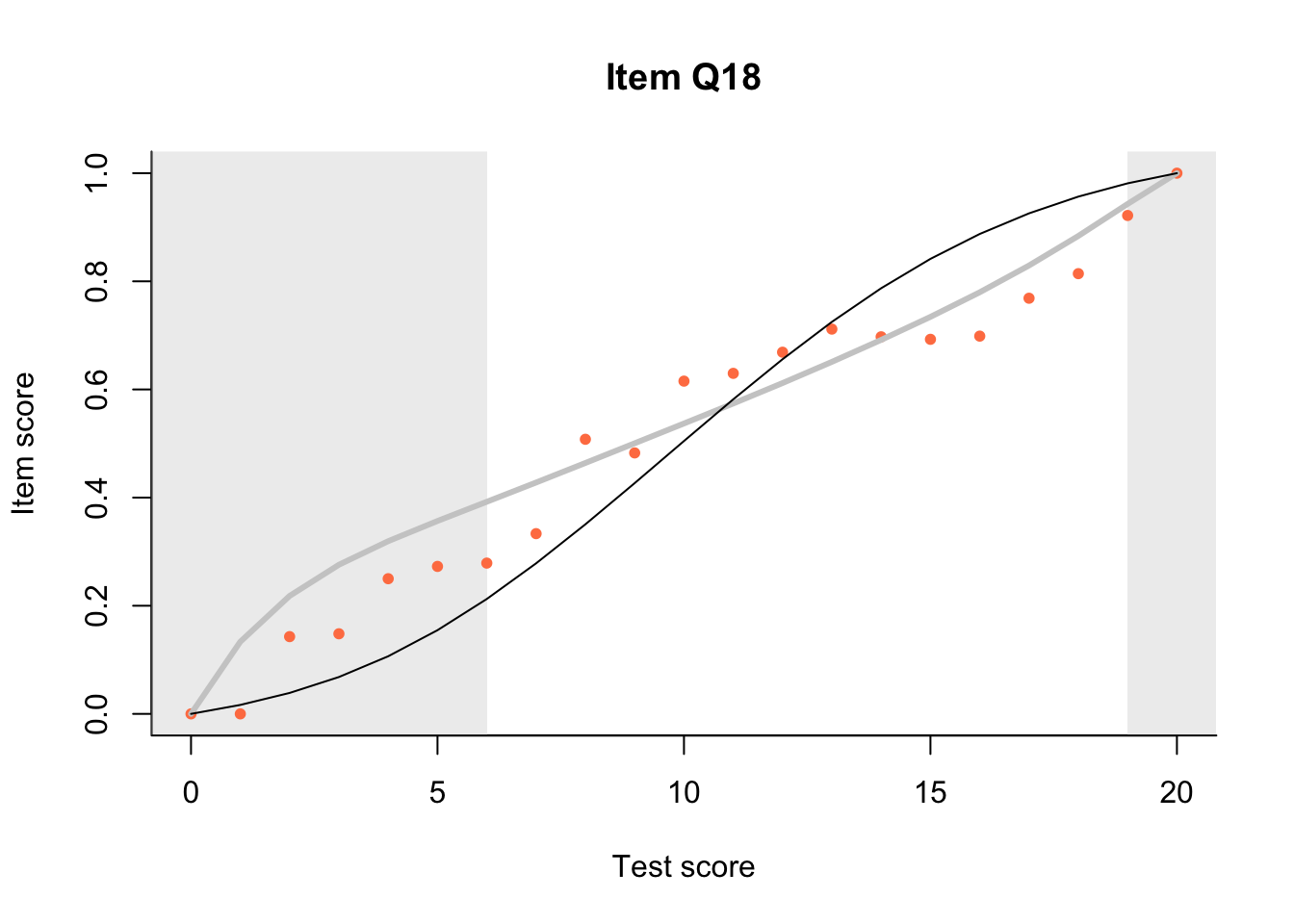
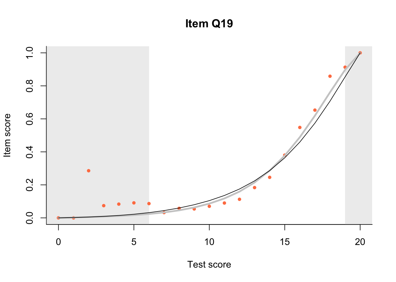
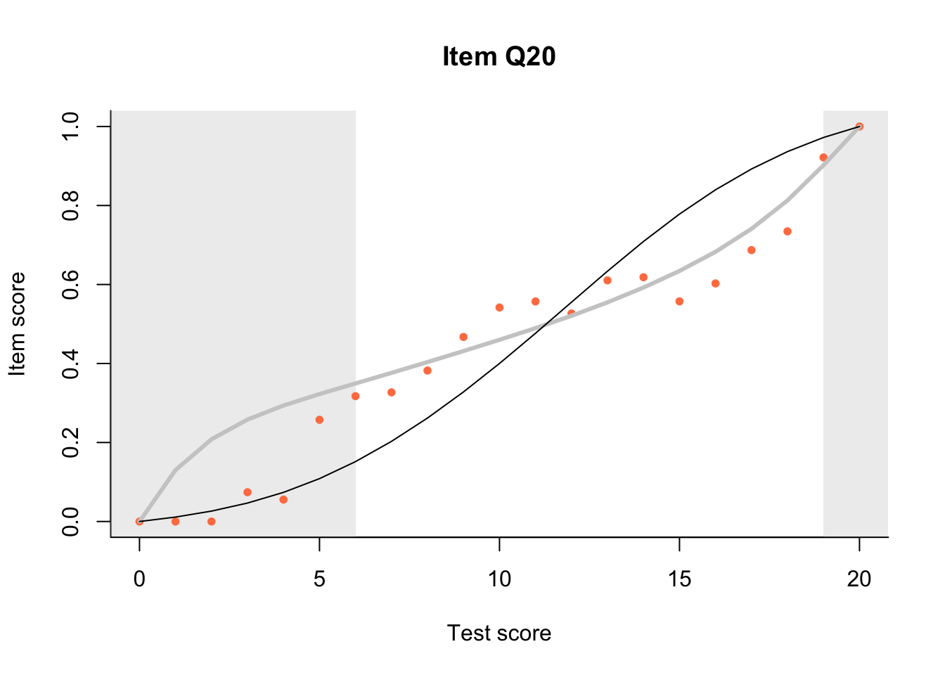
Look at Item Characteristic Plots for all items. There are three item-test regressions on the plot: the observed one, shown as pink dots; the interaction model, shown with a thick gray line; and the ENORM model, shown with a thin black line. (ENORM=RASCH for dichotomous models)
add_booklet(db, responses, "y7") no column `person_id` provided, automatically generating unique person id's$items
[1] "Q1" "Q2" "Q3" "Q4" "Q5" "Q6" "Q7" "Q8" "Q9" "Q10" "Q11" "Q12"
[13] "Q13" "Q14" "Q15" "Q16" "Q17" "Q18" "Q19" "Q20"
$person_properties
[1] "gender"
$columns_ignored
[1] "id" "dob" "yg" "missing" "Q1_score" "Q2_score"
[7] "Q3_score" "Q4_score" "Q5_score" "Q6_score" "Q7_score" "Q8_score"
[13] "Q9_score" "Q10_score" "Q11_score" "Q12_score" "Q13_score" "Q14_score"
[19] "Q15_score" "Q16_score" "Q17_score" "Q18_score" "Q19_score" "Q20_score"get_booklets(db) booklet_id n_items n_persons booklet_max_score
1 y7 20 3061 20m = fit_inter(db, booklet_id=='y7')
n_items <- nrow(keys)
for(i in 1:n_items){
plot(m, keys$item_id[i], show.observed=TRUE)
}
tt = tia_tables(db)
knitr::kable(tt$items, digits=2)| booklet_id | item_id | mean_score | sd_score | max_score | pvalue | rit | rir | n_persons |
|---|---|---|---|---|---|---|---|---|
| y7 | Q1 | 0.95 | 0.23 | 1 | 0.95 | 0.33 | 0.28 | 3061 |
| y7 | Q10 | 0.78 | 0.41 | 1 | 0.78 | 0.49 | 0.41 | 3061 |
| y7 | Q11 | 0.82 | 0.39 | 1 | 0.82 | 0.44 | 0.35 | 3061 |
| y7 | Q12 | 0.59 | 0.49 | 1 | 0.59 | 0.58 | 0.49 | 3061 |
| y7 | Q13 | 0.66 | 0.47 | 1 | 0.66 | 0.42 | 0.31 | 3061 |
| y7 | Q14 | 0.72 | 0.45 | 1 | 0.72 | 0.50 | 0.41 | 3061 |
| y7 | Q15 | 0.18 | 0.38 | 1 | 0.18 | 0.45 | 0.37 | 3061 |
| y7 | Q16 | 0.30 | 0.46 | 1 | 0.30 | 0.54 | 0.45 | 3061 |
| y7 | Q17 | 0.55 | 0.50 | 1 | 0.55 | 0.41 | 0.30 | 3061 |
| y7 | Q18 | 0.62 | 0.48 | 1 | 0.62 | 0.35 | 0.23 | 3061 |
| y7 | Q19 | 0.26 | 0.44 | 1 | 0.26 | 0.56 | 0.48 | 3061 |
| y7 | Q2 | 0.92 | 0.27 | 1 | 0.92 | 0.37 | 0.31 | 3061 |
| y7 | Q20 | 0.55 | 0.50 | 1 | 0.55 | 0.33 | 0.21 | 3061 |
| y7 | Q3 | 0.66 | 0.47 | 1 | 0.66 | 0.50 | 0.41 | 3061 |
| y7 | Q4 | 0.93 | 0.25 | 1 | 0.93 | 0.34 | 0.29 | 3061 |
| y7 | Q5 | 0.90 | 0.31 | 1 | 0.90 | 0.38 | 0.31 | 3061 |
| y7 | Q6 | 0.39 | 0.49 | 1 | 0.39 | 0.61 | 0.53 | 3061 |
| y7 | Q7 | 0.31 | 0.46 | 1 | 0.31 | 0.56 | 0.47 | 3061 |
| y7 | Q8 | 0.33 | 0.47 | 1 | 0.33 | 0.60 | 0.52 | 3061 |
| y7 | Q9 | 0.59 | 0.49 | 1 | 0.59 | 0.61 | 0.52 | 3061 |
17.4 Analysis
17.4.1 Guessing
The left hand curtain gives us an idea of guessing. By default, they are drawn at the 5th and the 95th percentile of the observed test scores, highlighting the central 90% of the data. The left curtain highlights the likely item score for the pupils at the 95th percentile. From examination of the ICCs, which items are prone to guessing?
17.4.2 Model fit
Which items seem to fit the Rasch model less well? Which restriction of the Rasch model do these items highlight? How can the fit of the model be improved?
close_project(db)