Item Response Theory (IRT) uses a mathematical function to model the probability of a person’s success on a test item, given their level of ability and the item’s difficulty. The function should be bounded by 0 and 1, meaning that it models probability. It should also be increasing, indicating that the chance of success is higher for people with higher abilities. The function should have an S-shaped curve, with the left side close to 0 and the right side close to 1 but not exceeding it.
There are several mathematical functions that fit this shape, such as cumulative distribution functions (cdf) or ogives. Examples of ogives that have been used in IRT include the logistic ogive and the normal ogive, but for the purposes of this discussion, we will focus on the logistic ogive. The logistic ogive is a function that can be used to model the probability of success on an item and has the desired S-shaped curve, making it a commonly used function in IRT.
The Rasch item response model (Rasch 1960) uses the following function to model the probability of success on an item with item difficulty δ and ability θ
── Conflicts ────────────────────────────────────────── tidyverse_conflicts() ──
✖ dplyr::filter() masks stats::filter()
✖ dplyr::lag()    masks stats::lag()
ℹ Use the conflicted package (<http://conflicted.r-lib.org/>) to force all conflicts to become errors
# Calculate Rasch model probabilitydelta <-0#item difficulty is 0.6theta <-0#person ability is 1.0prob <-exp(theta-delta)/(1+exp(theta-delta))prob
[1] 0.5
Change the values of delta and theta, and observe how prob changes. In particular, try values when (1) delta = theta, (2) delta > theta, and (3) delta < theta. What happens when theta is very high, and when theta is very low?
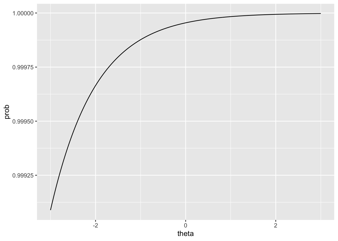
We will plot the probability as a function of θ.
#Calculate prob as a function the thetaid =1# item iddelta <--10#item difficulty is 1theta <-seq(-3,3,0.01) #a vector of theta from -3 to 3 in steps of 0.01prob_function <-function(theta, delta){return (exp(theta-delta)/(1+exp(theta-delta)))}probs <-tibble(id = id, delta=delta,theta=theta)probs <- probs %>%mutate(prob =prob_function(theta, delta))p <-ggplot(probs, aes(x=theta, y=prob))p <- p +geom_line()print(p)
Figure 15.1: Item Characteristic Curve
15.1 Exercise
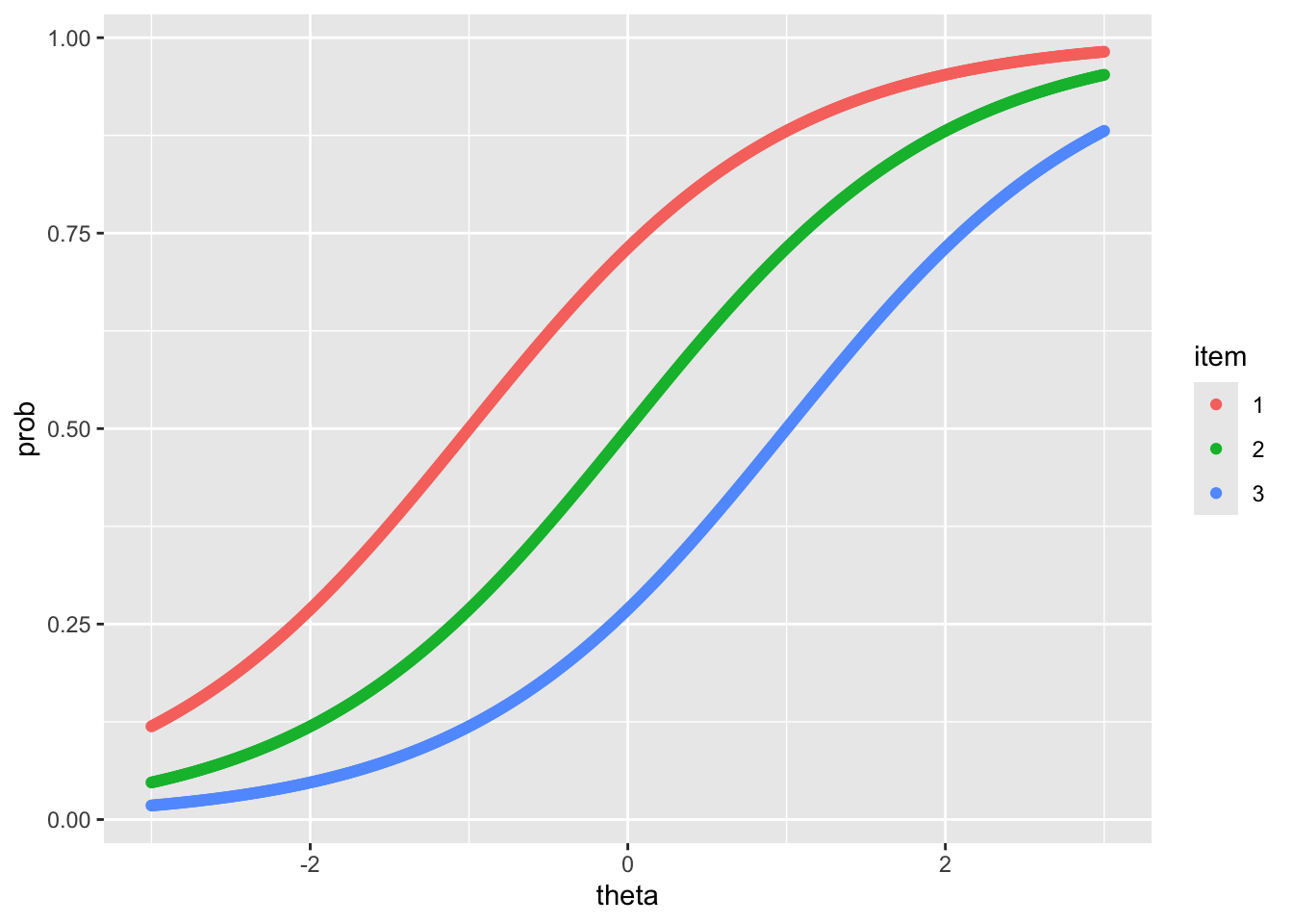
As an exercise, plot three ICC for three items with (1) δ = −1, (2) δ = 0, and (3) δ = 1.
#Calculate prob as a function the thetaid =1# item iddelta <--1#item difficulty is 1theta <-seq(-3,3,0.01) #a vector of theta from -3 to 3 in steps of 0.01prob_function <-function(theta, delta){return (exp(theta-delta)/(1+exp(theta-delta)))}probs <-tibble(id = id, delta=delta,theta=theta)probs <- probs %>%mutate(prob =prob_function(theta, delta))item1 <-tibble(id =1, delta=-1,theta=theta)item2 <-tibble(id=2, delta=0, theta=theta)item3 <-tibble(id=3, delta=1, theta=theta)items <-bind_rows(item1, item2, item3)items <- items %>%mutate(item=factor(id))items_probs <- items %>%mutate(prob =prob_function(theta, delta))p <-ggplot(items_probs, aes(x=theta, y=prob,colour=item))p <- p +geom_point()print(p)
Figure 15.2: Item Characteristic Curves
See if you can work out how to plot the three graphs using different colors. Can you easily identify the ICC of the easier item?
15.2 Theta Scale Unit
The θ scale is in “logit” unit. Answer the following questions, assuming the item responses follow a Rasch model:
What is the probability of success when θ = δ?
What is the probability of success when θ = 2 logit and δ = 1 logit?
What is the probability of success when a person’s ability is 1.5 logit higher than the item difficulty?
What is the probability of success when a person’s ability is 0.6 logit lower than the item difficulty?
Is the following statement TRUE or FALSE: The difference in logit between a person’s ability and an item’s difficulty determines the probability of success, irrespective of what the ability is.
Consider CTT item difficulty and person ability, can we say anything about the likelihood of success for a person who scored 80% on a test, on an item where 80% of the candidates answered correctly?
Andrich, David, and Ida Marais. 2019. “The Idea of Measurement.” In A Course in Rasch Measurement Theory, 3–11. Springer Nature Singapore. https://doi.org/10.1007/978-981-13-7496-8_1.
Bond, Trevor G., Zi Yan, and Moritz Heene. 2020. Applying the Rasch Model: Fundamental Measurement in the Human Sciences. Routledge. https://doi.org/10.4324/9780429030499.
Cappelleri, Jason Lundy, J. C. 2014. “Overview of Classical Test Theory and Item Response Theory for the Quantitative Assessment of Items in Developing Patient-Reported Outcomes Measures.”Clinical Therapeutics 36 (5): 648–62. https://doi.org/https://doi.org/10.1016/j.clinthera.2014.04.006.
Cronbach, Lee J. 1951. “Coefficient Alpha and the Internal Structure of Tests.”Psychometrika 16 (3): 297–334. https://doi.org/10.1007/bf02310555.
Goldstein, H., and Steve Blinkhorn. 1982. “The Rasch Model Still Does Not Fit.”British Educational Research Journal 8 (2): 167–70. https://doi.org/10.1080/0141192820080207.
Lord, Frederic M, and Melvin R Novick. 2008. Statistical Theories of Mental Test Scores. IAP.
McNeish, Daniel. 2018. “Thanks Coefficient Alpha, We’ll Take It from Here.”Psychological Methods 23 (3): 412–33. https://doi.org/10.1037/met0000144.
Panayides, Panayiotis, Colin Robinson, and Peter Tymms. 2010. “The Assessment Revolution That Has Passed England by: Rasch Measurement.”British Educational Research Journal 36 (4): 611–26. https://doi.org/10.1080/01411920903018182.
Sijtsma, Klaas. 2008. “On the Use, the Misuse, and the Very Limited Usefulness of Cronbach’s Alpha.”Psychometrika 74 (1): 107–20. https://doi.org/10.1007/s11336-008-9101-0.
Wright, Benjamin D, and Magdalena Mok. 2000. “Rasch Models Overview.”Journal of Applied Measurement 1 (1): 83–106.