rm(list=ls())
library(tidyverse)
library(ggplot2)
library(sirt)
decisions <- read_csv('data/decisions-1.csv')
persons <- read_csv('data/persons-1.csv')
glimpse(decisions)
glimpse(persons)30 Comparative Judgement Practical
Create a new Comparative Judgement task on www.nomoremarking.com and upload 8 pdfs with the numbers 1 to 8. Judge the numbers 80 times and download the decisions file.
30.1 Fitting the Bradley-Terry Model
# get the person ids and their first names
persons <- persons %>%
  select(Code, `First Name`) %>%
  rename(id = Code, name = `First Name`)

# go through the decisions and add a column with the name of the person who was chosen or not chosen in each case
decisions <- decisions %>% left_join(persons, by = c('chosen' = 'id')) %>%
  rename(chosenName = name) %>%
  left_join(persons, by = c('notChosen' = 'id')) %>%
  rename(notChosenName = name)

# mutate chosenName and notChosenName to be factors
decisions <- decisions %>%
  mutate(chosenName = factor(chosenName), notChosenName = factor(notChosenName))

# create a name for each judge
decisions <- decisions %>% mutate(
    judge = paste0('judge_', judgeName)
)

# get a vector of judges
judges <- decisions %>% pull(judge)

# format for the btm model
decisions <- decisions %>%
  select(chosenName, notChosenName) %>%
  mutate(result = 1)

# the package doesn't like tibbles?
decisions <- as.data.frame(decisions)
mod1 <- btm(decisions, judge=judges, fix.eta = 0, ignore.ties = TRUE, eps = 0.3)
30.2 Explore the model results
See https://alexanderrobitzsch.github.io/sirt/reference/btm.html
30.2.1 Reliability
# The mle reliability, also known as separation reliability
print(mod1$mle.rel)
[1] 0.890099330.2.2 Person parameters
# The person parameters
knitr::kable(mod1$effects, digits = 2)| individual | id | Ntot | N1 | ND | N0 | raw | score | propscore | theta | se.theta | outfit | infit | |
|---|---|---|---|---|---|---|---|---|---|---|---|---|---|
| 8 | 8 | 8 | 24 | 24 | 0 | 0 | 24 | 23.70 | 0.99 | 6.42 | 1.86 | 0.01 | 0.05 |
| 7 | 7 | 7 | 21 | 17 | 0 | 4 | 17 | 16.81 | 0.80 | 3.56 | 1.38 | 0.04 | 0.19 |
| 6 | 6 | 6 | 20 | 16 | 0 | 4 | 16 | 15.82 | 0.79 | 2.65 | 1.15 | 0.05 | 0.19 |
| 5 | 5 | 5 | 20 | 12 | 0 | 8 | 12 | 11.94 | 0.60 | 0.81 | 1.04 | 0.06 | 0.13 |
| 4 | 4 | 4 | 20 | 7 | 0 | 13 | 7 | 7.09 | 0.35 | -0.91 | 1.17 | 0.05 | 0.16 |
| 3 | 3 | 3 | 19 | 4 | 0 | 15 | 4 | 4.17 | 0.22 | -2.01 | 1.16 | 0.05 | 0.15 |
| 2 | 2 | 2 | 21 | 3 | 0 | 18 | 3 | 3.21 | 0.15 | -4.10 | 1.21 | 0.04 | 0.10 |
| 1 | 1 | 1 | 21 | 0 | 0 | 21 | 0 | 0.30 | 0.01 | -6.41 | 1.92 | 0.02 | 0.09 |
30.2.3 Judge fit
# The judge fit
# Fit statistics (outfit and infit) for judges if judge is provided. In addition, average agreement of the rating with the mode of the ratings is calculated for each judge (at least three ratings per dyad has to be available for computing the agreement)
knitr::kable(mod1$fit_judges, digits = 2)| judge | outfit | infit | agree | |
|---|---|---|---|---|
| judge_1 | judge_1 | 0.06 | 0.23 | 1 |
| judge_2 | judge_2 | 0.02 | 0.09 | 1 |
| judge_3 | judge_3 | 0.05 | 0.14 | 1 |
| judge_4 | judge_4 | 0.04 | 0.11 | 1 |
| judge_5 | judge_5 | 0.02 | 0.13 | 1 |
| judge_6 | judge_6 | 0.08 | 0.27 | 1 |
| judge_7 | judge_7 | 0.03 | 0.08 | 1 |
| judge_8 | judge_8 | 0.03 | 0.08 | 1 |
| judge_9 | judge_9 | 0.03 | 0.07 | 1 |
30.2.4 Visualise the person parameters (model effects) along with the standard error
# plot the model effects with the standard errors
# add a column to the person parameters with the upper and lower limits using 1.96 * standard error
effects <- mod1$effects %>%
  mutate(
    lower = theta - 1.96 * se.theta,
    upper = theta + 1.96 * se.theta
  )

p <- ggplot(effects, aes(x = individual, y = theta)) +
  geom_point() +
  geom_errorbar(aes(ymin = lower, ymax = upper), width = 0.2) +
  theme_bw() +
  labs(x = 'Person parameter', y = 'Person')
print(p)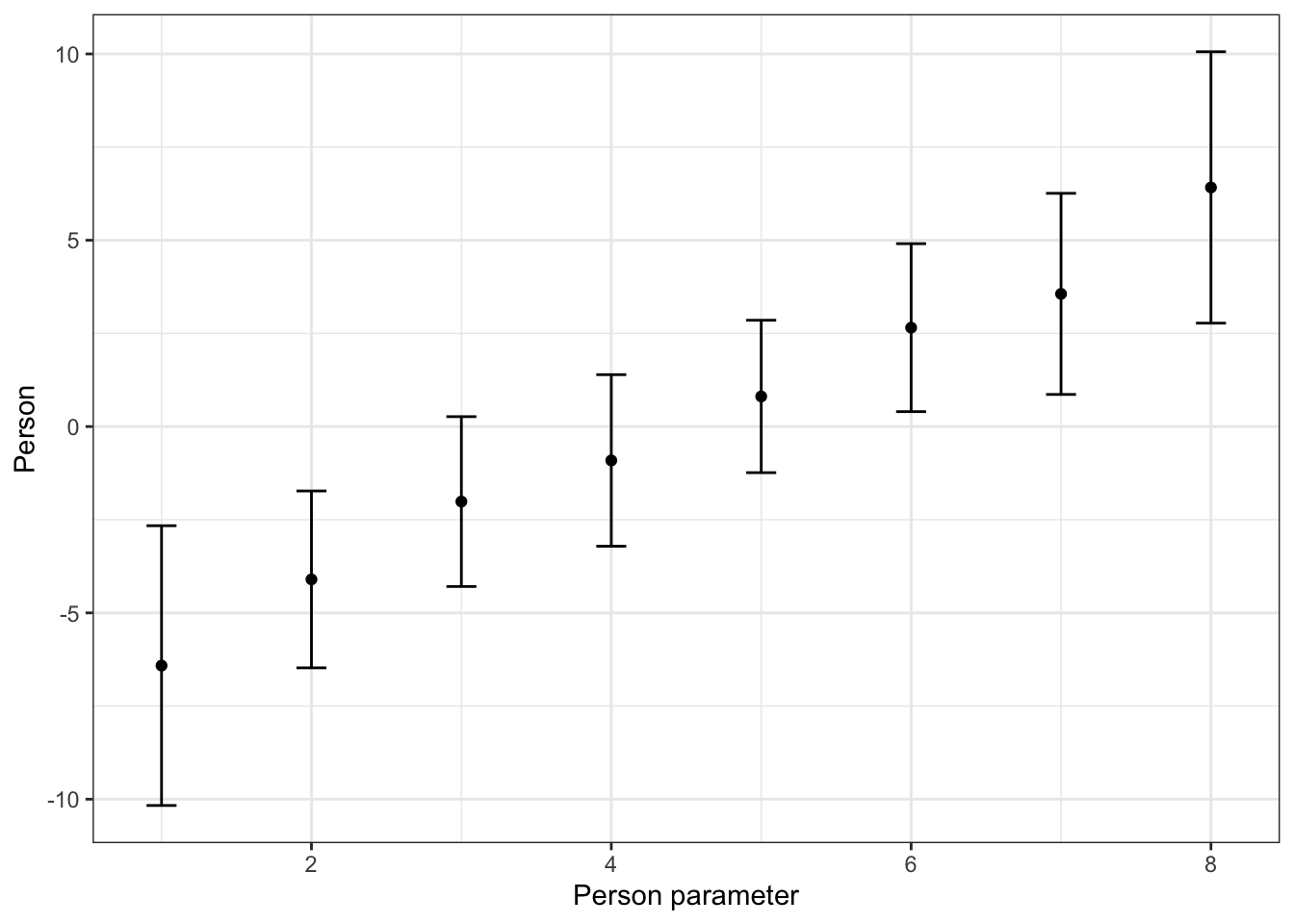
30.2.5 Inspect the model probabilities
30.2.6 What is p1? p0? pD?
head(mod1$probs) p1 p0 pD
[1,] 0.9963473 0.0036526689 6.100379e-45
[2,] 0.9998848 0.0001151765 1.085183e-45
[3,] 0.7509258 0.2490741530 4.373299e-44
[4,] 0.9906881 0.0093119089 9.712569e-45
[5,] 0.9099456 0.0900544355 2.894720e-44
[6,] 0.9959516 0.0040483851 6.421054e-4530.3 Extension exercises
- Try some less accurate judging. Note the impact on the model parameters.
- Can you recreate the model probabilities?