rm(list=ls())
library(tidyverse)
# load in the dataset
responses <- read_csv('data/responses.csv')6 Descriptive Data
6.1 Item facility or mean item score
In the special case of dichotomous items, scored “0” for one response and “1” for the other, the proportion of respondents in a sample who select the response choice scored “1” is equivalent to the mean item response. Items for which everyone gives the same response are uninformative because they do not differentiate between individuals. In contrast, dichotomous items that yield about an equal number of people (50%) selecting each of the two response options provide the best differentiation between individuals in the sample overall (Cappelleri (2014)).
# select all the columns with _score as the suffix and store as a tibble
items <- responses %>% select(ends_with('_score'))

# pivot the items longer for analysis
items <- items %>% pivot_longer(cols=starts_with('Q'), names_to = 'item', values_to = 'score')

# create a summary table with item stats
item_stats <- items %>%
  group_by(item) %>%
  summarise(across(everything(),
  list(
    max = ~max(.x, na.rm = TRUE),
    n = ~sum(!is.na(.x)),
    mean = ~mean(.x, na.rm = TRUE),
    sd = ~sd(.x, na.rm = TRUE)))
)

item_stats <- item_stats %>% mutate(
    item_name = factor(item, levels=paste('Q',1:20, '_score',sep=''),labels = paste0('Q',1:20),ordered = TRUE)
)

item_stats <- item_stats %>% arrange(item_name) %>%
    select(
        item_name,
        score_max,
        score_n,
        score_mean,
        score_sd
    ) %>% rename(
        Item = item_name,
        Max = score_max,
        N = score_n,
        Mean = score_mean,
        SD = score_sd
    )

# display the summary table
knitr::kable(item_stats, digits=2)| Item | Max | N | Mean | SD |
|---|---|---|---|---|
| Q1 | 1 | 3049 | 0.95 | 0.22 |
| Q2 | 1 | 3039 | 0.93 | 0.25 |
| Q3 | 1 | 3049 | 0.66 | 0.47 |
| Q4 | 1 | 3050 | 0.94 | 0.24 |
| Q5 | 1 | 3050 | 0.90 | 0.30 |
| Q6 | 1 | 3047 | 0.39 | 0.49 |
| Q7 | 1 | 3037 | 0.31 | 0.46 |
| Q8 | 1 | 3039 | 0.33 | 0.47 |
| Q9 | 1 | 3046 | 0.59 | 0.49 |
| Q10 | 1 | 3046 | 0.79 | 0.41 |
| Q11 | 1 | 3043 | 0.82 | 0.38 |
| Q12 | 1 | 3040 | 0.59 | 0.49 |
| Q13 | 1 | 3036 | 0.67 | 0.47 |
| Q14 | 1 | 3045 | 0.72 | 0.45 |
| Q15 | 1 | 3042 | 0.18 | 0.38 |
| Q16 | 1 | 3039 | 0.30 | 0.46 |
| Q17 | 1 | 3039 | 0.55 | 0.50 |
| Q18 | 1 | 3022 | 0.63 | 0.48 |
| Q19 | 1 | 3036 | 0.26 | 0.44 |
| Q20 | 1 | 3034 | 0.55 | 0.50 |
6.2 What do we learn from the item facility table?
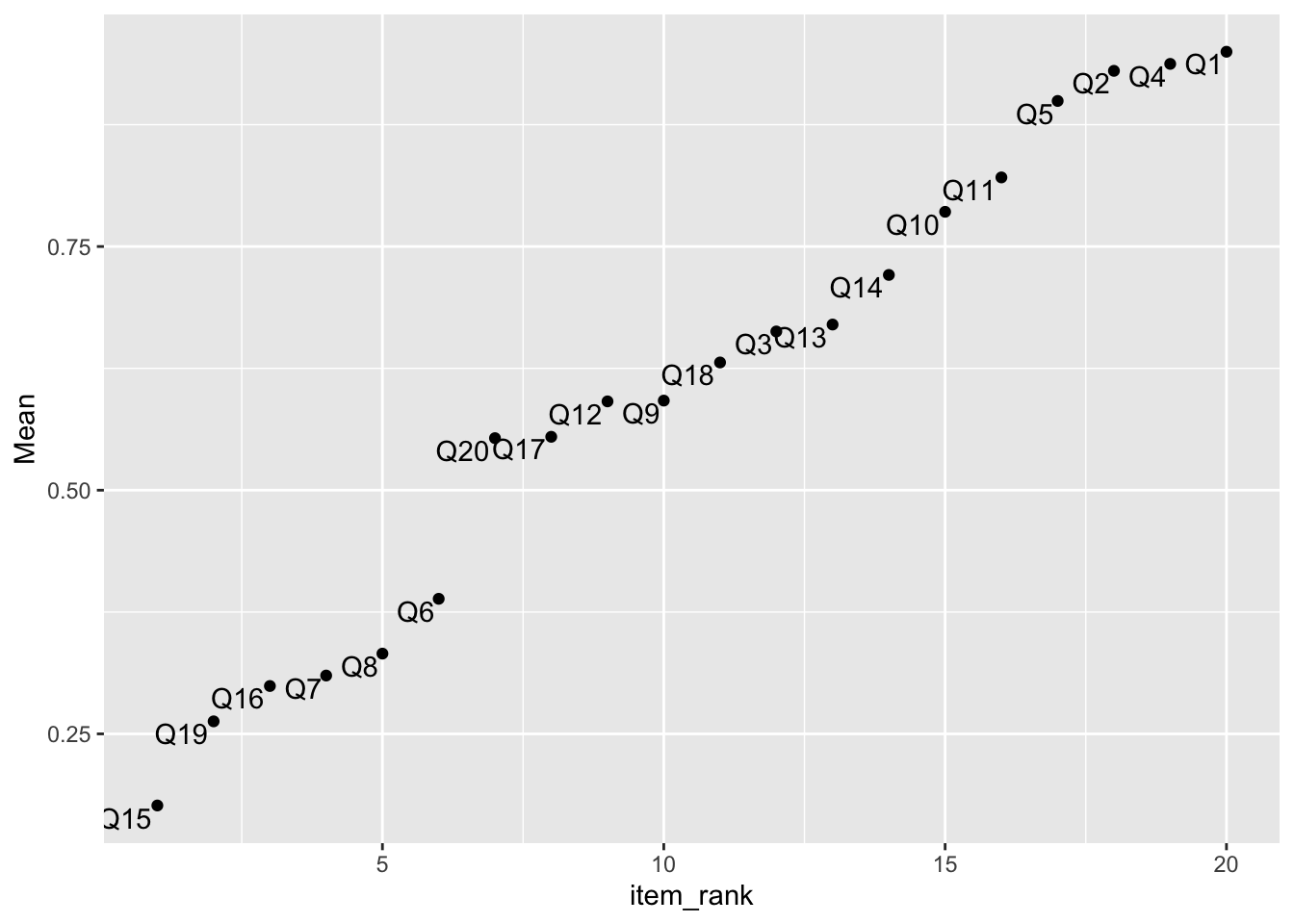
6.3 Plot the items by item difficulty in ascending order of difficulty
item_stats <- item_stats %>% arrange(Mean) %>% mutate (item_rank = row_number())
# plot the item_stats by item difficulty in ascending order of difficulty
ggplot(item_stats, aes(x=item_rank, y=Mean)) +
    geom_point()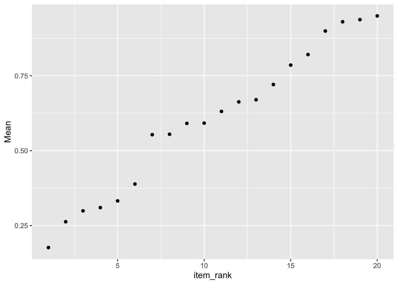
# label the items
ggplot(item_stats, aes(x=item_rank, y=Mean)) +
    geom_point() +
    geom_text(aes(x=item_rank,y=Mean,label=Item), hjust=1.1, vjust=1.1)