rm(list=ls())
library(tidyverse)
# load in the dataset
responses <- read_csv('data/responses.csv')

# sum across the columns with _score_ in the name and add to a new column called total.
# make sure to ignore missing values
# https://dplyr.tidyverse.org/articles/rowwise.html
# https://dplyr.tidyverse.org/reference/pick.html?q=pick#ref-usage
responses <- responses %>% mutate(total = rowSums(pick(ends_with("_score")), na.rm = TRUE))9 Correlations
9.1 Item Total Correlations
Item total correlations, are generally used as supporting evidence for the reliability of test forms. Items may be excluded from a test form if they have a poor correlation to the total score. The item total correlation is the correlation between the item score and the total score.
# correlate each item score with the total score
# note that this function includes the studied item score in the total score for simplicity, but normally the item score would be excluded from the total score, see https://personality-project.org/r/html/alpha.html
item_total_r <- responses %>%
  select(ends_with("_score")) %>%
  mutate(total = responses$total) %>%
  gather(key = "item", value = "score", -total) %>%
  mutate(item = str_remove(item, "_score")) %>%
  group_by(item) %>%
  summarise(mean = mean(score, na.rm=T), correlation = cor(score, total, use = "pairwise.complete.obs")) %>%
  arrange(desc(correlation))

knitr::kable(item_total_r, digits = 2)| item | mean | correlation |
|---|---|---|
| Q6 | 0.39 | 0.62 |
| Q8 | 0.33 | 0.60 |
| Q9 | 0.59 | 0.60 |
| Q12 | 0.59 | 0.58 |
| Q19 | 0.26 | 0.56 |
| Q7 | 0.31 | 0.56 |
| Q16 | 0.30 | 0.54 |
| Q3 | 0.66 | 0.50 |
| Q14 | 0.72 | 0.50 |
| Q10 | 0.79 | 0.48 |
| Q15 | 0.18 | 0.45 |
| Q11 | 0.82 | 0.43 |
| Q13 | 0.67 | 0.41 |
| Q17 | 0.55 | 0.41 |
| Q2 | 0.93 | 0.37 |
| Q5 | 0.90 | 0.37 |
| Q18 | 0.63 | 0.34 |
| Q4 | 0.94 | 0.34 |
| Q20 | 0.55 | 0.32 |
| Q1 | 0.95 | 0.32 |
9.2 Discussion
Is there a relationship between item difficulty and item total correlation? Can you plot this relationship? Can you see any issues with excluding items based on item total correlation?
9.3 Inter-item Correlations
# Correlate each item score with every other item score
# https://corrr.tidymodels.org/
library(corrr)
x1 <- responses %>%
  select(ends_with("_score")) %>%
  correlate() %>%
  rearrange() %>%
  shave()
Correlation computed with
• Method: 'pearson'
• Missing treated using: 'pairwise.complete.obs'fashion(x1) term Q1_score Q4_score Q2_score Q5_score Q11_score Q18_score Q10_score
1 Q1_score
2 Q4_score .31
3 Q2_score .34 .27
4 Q5_score .29 .33 .31
5 Q11_score .18 .22 .23 .19
6 Q18_score .10 .11 .12 .11 .13
7 Q10_score .23 .23 .24 .23 .26 .18
8 Q20_score .08 .09 .11 .08 .13 .16 .09
9 Q13_score .15 .14 .15 .13 .19 .16 .15
10 Q14_score .18 .14 .20 .21 .23 .12 .31
11 Q3_score .20 .20 .22 .20 .17 .11 .19
12 Q17_score .08 .12 .12 .10 .12 .06 .17
13 Q9_score .11 .16 .16 .18 .26 .10 .30
14 Q12_score .12 .14 .12 .13 .22 .11 .25
15 Q6_score .10 .11 .14 .17 .16 .11 .17
16 Q8_score .09 .11 .07 .09 .19 .08 .25
17 Q7_score .07 .03 .09 .09 .10 .07 .11
18 Q15_score .00 .01 .04 .04 .04 .09 .07
19 Q19_score .06 .06 .07 .06 .10 .10 .15
20 Q16_score .02 .03 .05 .04 .12 .09 .12
Q20_score Q13_score Q14_score Q3_score Q17_score Q9_score Q12_score Q6_score
1
2
3
4
5
6
7
8
9 .15
10 .10 .18
11 .11 .18 .21
12 .07 .09 .22 .13
13 .08 .19 .28 .23 .17
14 .08 .18 .24 .23 .17 .38
15 .09 .18 .23 .33 .14 .32 .33
16 .07 .19 .24 .22 .18 .43 .38 .40
17 .09 .14 .17 .27 .15 .27 .28 .52
18 .09 .06 .11 .13 .17 .23 .19 .30
19 .11 .11 .17 .19 .18 .31 .31 .41
20 .09 .07 .16 .19 .23 .30 .32 .33
Q8_score Q7_score Q15_score Q19_score Q16_score
1
2
3
4
5
6
7
8
9
10
11
12
13
14
15
16
17 .39
18 .31 .35
19 .38 .40 .42
20 .37 .35 .46 .46 stretch(x1, na.rm = TRUE) %>% arrange(r)# A tibble: 190 × 3
x y r
<chr> <chr> <dbl>
1 Q1_score Q15_score 0.00206
2 Q4_score Q15_score 0.0119
3 Q1_score Q16_score 0.0187
4 Q4_score Q16_score 0.0268
5 Q4_score Q7_score 0.0323
6 Q5_score Q15_score 0.0370
7 Q11_score Q15_score 0.0385
8 Q5_score Q16_score 0.0435
9 Q2_score Q15_score 0.0437
10 Q2_score Q16_score 0.0450
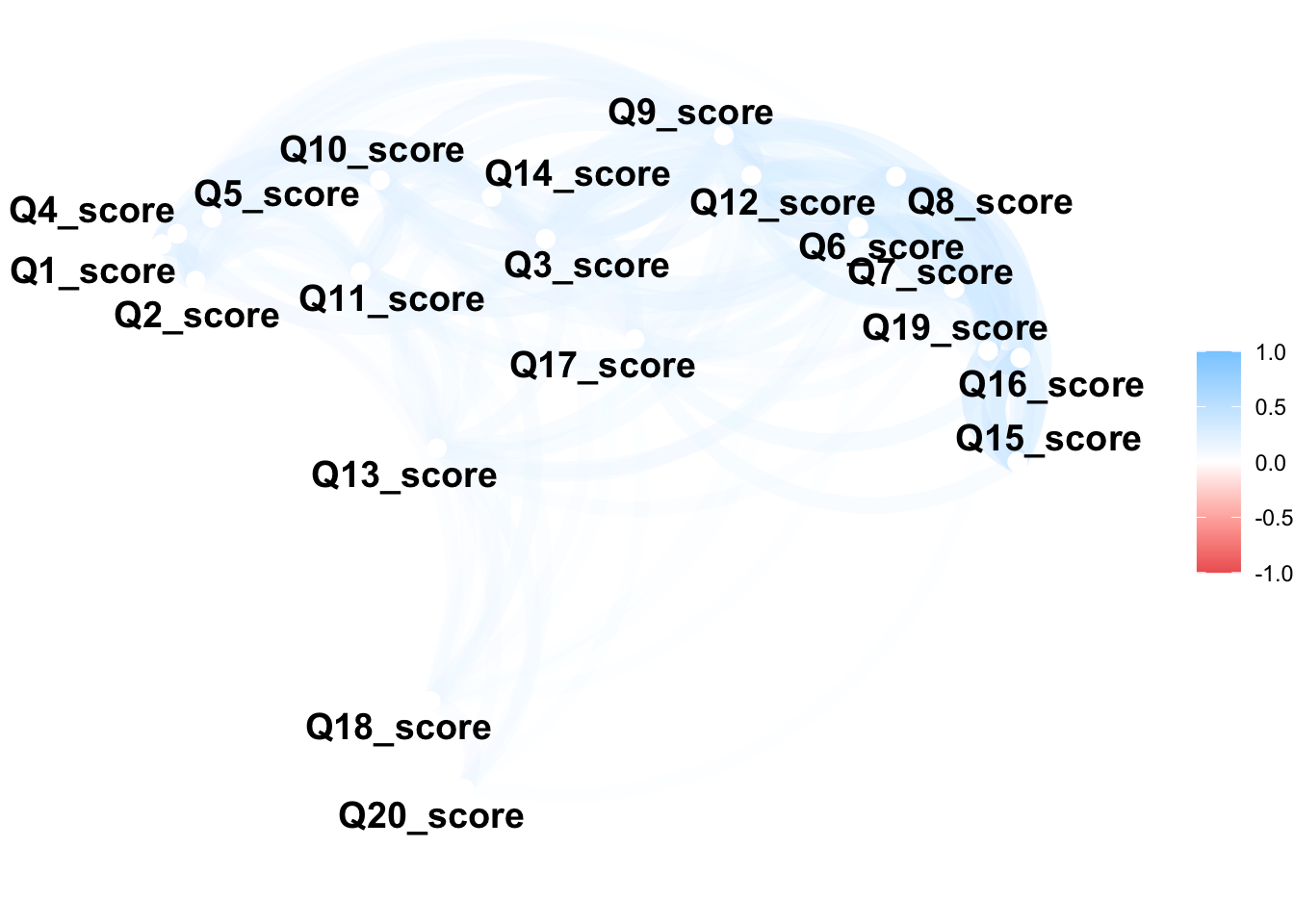
# ℹ 180 more rows9.4 Try some visulations suggested by the package eg. the network plot
x2 <- responses %>%
  select(ends_with("_score")) %>%
  correlate()
Correlation computed with
• Method: 'pearson'
• Missing treated using: 'pairwise.complete.obs'x2 %>% network_plot(min_cor = .1)