18  Item Difficulty and Person Ability

A more traditional approach to the Rasch model is operationalised in the package TAM https://alexanderrobitzsch.github.io/TAM/

18.1 Fitting the Rasch model with TAM

rm(list=ls())  #remove all variables in the R environment
library(tidyverse)
library(TAM)  #load the package TAM so we can use the functions in TAM

# load in the dataset
responses <- read_csv('data/responses.csv')
# keep the scores
responses <- responses %>% select(ends_with('score'))

#run a joint maximum likelihood estimation of the Rasch model
mod1 <- tam.jml(responses)

#All the results of the Rasch analysis are stored in the object called "mod1"
summary(mod1)  #see a summary of the results

------------------------------------------------------------
TAM 4.2-21 (2024-02-19 18:52:08) 
R version 4.2.2 (2022-10-31) aarch64, darwin20 | nodename=Christophers-MacBook-Air.local | login=root 

Start of Analysis: 2024-04-18 09:47:43 
End of Analysis: 2024-04-18 09:47:43 
Time difference of 0.09173584 secs
Computation time: 0.09173584 

Joint Maximum Likelihood Estimation in TAM 

IRT Model
Call:
tam.jml(resp = responses)

------------------------------------------------------------
Number of iterations = 10 

Deviance = 50209.81  | Log Likelihood = -25104.9 
Number of persons = 3061 
Number of items = 20 
constraint = cases 
bias = TRUE 
------------------------------------------------------------
Person Parameters xsi
M = 0 
SD = 1.61 
------------------------------------------------------------
Item Parameters xsi
               item    N     M xsi.item AXsi_.Cat1 B.Cat1.Dim1
Q1_score   Q1_score 3049 0.950   -3.593     -3.593           1
Q2_score   Q2_score 3039 0.930   -3.217     -3.217           1
Q3_score   Q3_score 3049 0.663   -0.972     -0.972           1
Q4_score   Q4_score 3050 0.937   -3.341     -3.341           1
Q5_score   Q5_score 3050 0.899   -2.771     -2.771           1
Q6_score   Q6_score 3047 0.389    0.511      0.511           1
Q7_score   Q7_score 3037 0.310    0.997      0.997           1
Q8_score   Q8_score 3039 0.332    0.853      0.853           1
Q9_score   Q9_score 3046 0.592   -0.581     -0.581           1
Q10_score Q10_score 3046 0.786   -1.736     -1.736           1
Q11_score Q11_score 3043 0.821   -2.004     -2.004           1
Q12_score Q12_score 3040 0.591   -0.578     -0.578           1
Q13_score Q13_score 3036 0.670   -1.010     -1.010           1
Q14_score Q14_score 3045 0.721   -1.311     -1.311           1
Q15_score Q15_score 3042 0.177    2.044      2.044           1
Q16_score Q16_score 3039 0.299    1.067      1.067           1
Q17_score Q17_score 3039 0.555   -0.384     -0.384           1
Q18_score Q18_score 3022 0.631   -0.792     -0.792           1
Q19_score Q19_score 3036 0.263    1.320      1.320           1
Q20_score Q20_score 3034 0.553   -0.378     -0.378           1
------------------------------------------------------------
Item Parameters -A*Xsi
   xsi.label xsi.index    xsi se.xsi
1   Q1_score         1 -3.593  0.088
2   Q2_score         2 -3.217  0.076
3   Q3_score         3 -0.972  0.044
4   Q4_score         4 -3.341  0.080
5   Q5_score         5 -2.771  0.065
6   Q6_score         6  0.511  0.045
7   Q7_score         7  0.997  0.048
8   Q8_score         8  0.853  0.047
9   Q9_score         9 -0.581  0.043
10 Q10_score        10 -1.736  0.050
11 Q11_score        11 -2.004  0.053
12 Q12_score        12 -0.578  0.043
13 Q13_score        13 -1.010  0.044
14 Q14_score        14 -1.311  0.046
15 Q15_score        15  2.044  0.058
16 Q16_score        16  1.067  0.048
17 Q17_score        17 -0.384  0.043
18 Q18_score        18 -0.792  0.044
19 Q19_score        19  1.320  0.050
20 Q20_score        20 -0.378  0.043

#See specific results from the Rasch analysis
knitr::kable(mod1$item, digits=2)

	item	N	M	xsi.item	AXsi_.Cat1	B.Cat1.Dim1
Q1_score	Q1_score	3049	0.95	-3.59	-3.59	1
Q2_score	Q2_score	3039	0.93	-3.22	-3.22	1
Q3_score	Q3_score	3049	0.66	-0.97	-0.97	1
Q4_score	Q4_score	3050	0.94	-3.34	-3.34	1
Q5_score	Q5_score	3050	0.90	-2.77	-2.77	1
Q6_score	Q6_score	3047	0.39	0.51	0.51	1
Q7_score	Q7_score	3037	0.31	1.00	1.00	1
Q8_score	Q8_score	3039	0.33	0.85	0.85	1
Q9_score	Q9_score	3046	0.59	-0.58	-0.58	1
Q10_score	Q10_score	3046	0.79	-1.74	-1.74	1
Q11_score	Q11_score	3043	0.82	-2.00	-2.00	1
Q12_score	Q12_score	3040	0.59	-0.58	-0.58	1
Q13_score	Q13_score	3036	0.67	-1.01	-1.01	1
Q14_score	Q14_score	3045	0.72	-1.31	-1.31	1
Q15_score	Q15_score	3042	0.18	2.04	2.04	1
Q16_score	Q16_score	3039	0.30	1.07	1.07	1
Q17_score	Q17_score	3039	0.55	-0.38	-0.38	1
Q18_score	Q18_score	3022	0.63	-0.79	-0.79	1
Q19_score	Q19_score	3036	0.26	1.32	1.32	1
Q20_score	Q20_score	3034	0.55	-0.38	-0.38	1

head(mod1$WLE)

[1] -1.0960393  0.1223539 -1.0960393 -0.7940095 -2.8587070  0.3441501

mod1$WLEreliability

[1] 0.798689

18.2 Item and person summary statistics

# Item difficulty measures
summary(mod1$item1)

  xsi.label           xsi.index          xsi              se.xsi       
 Length:20          Min.   : 1.00   Min.   :-3.5930   Min.   :0.04278  
 Class :character   1st Qu.: 5.75   1st Qu.:-1.8032   1st Qu.:0.04400  
 Mode  :character   Median :10.50   Median :-0.6862   Median :0.04705  
                    Mean   :10.50   Mean   :-0.7937   Mean   :0.05286  
                    3rd Qu.:15.25   3rd Qu.: 0.5965   3rd Qu.:0.05408  
                    Max.   :20.00   Max.   : 2.0444   Max.   :0.08820  

# Person ability measures
summary(mod1$WLE)

    Min.  1st Qu.   Median     Mean  3rd Qu.     Max. 
-5.32508 -1.09604 -0.19013 -0.06263  0.79646  3.53328 

person_abilities <- tibble(theta=mod1$WLE)
p <- ggplot(person_abilities, aes(x=theta))
p <- p + geom_histogram(binwidth = 0.3)
p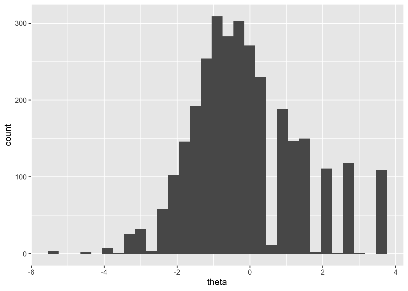

18.3 Item Characteristic Curves

plot(mod1)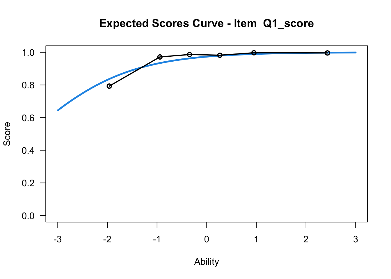

....................................................
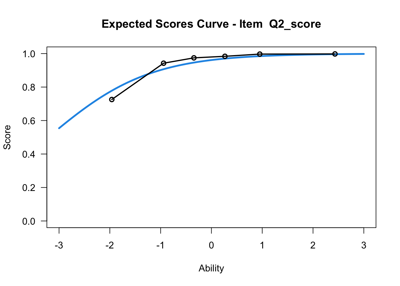
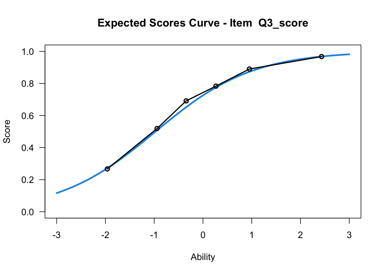
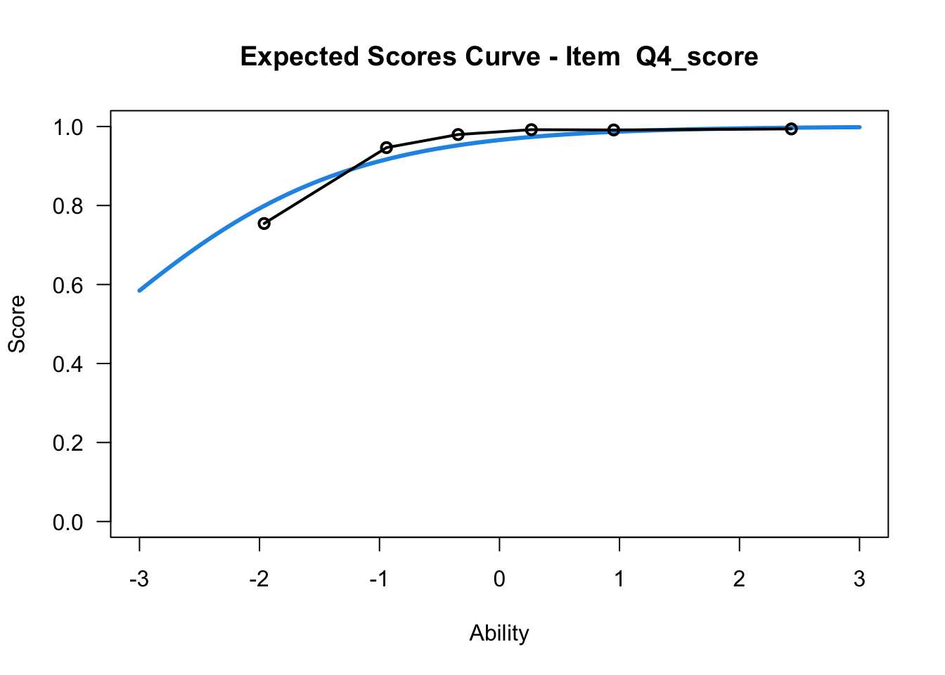
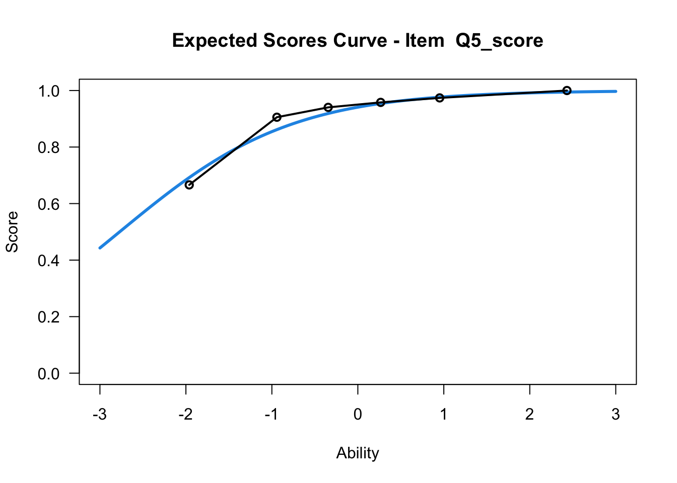
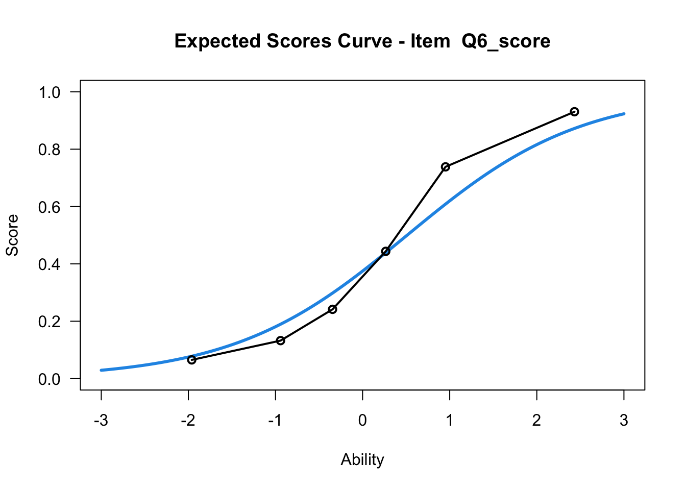
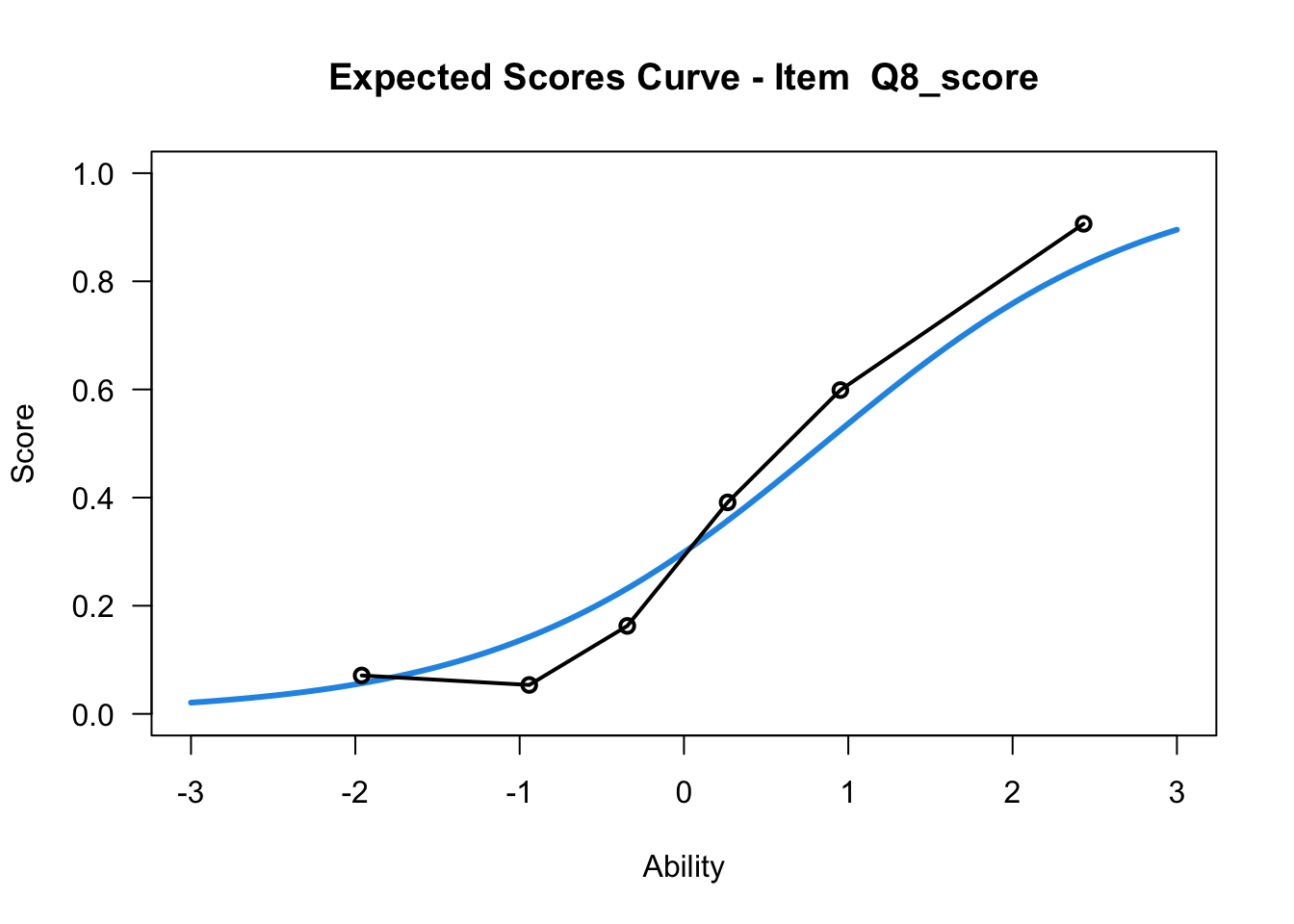
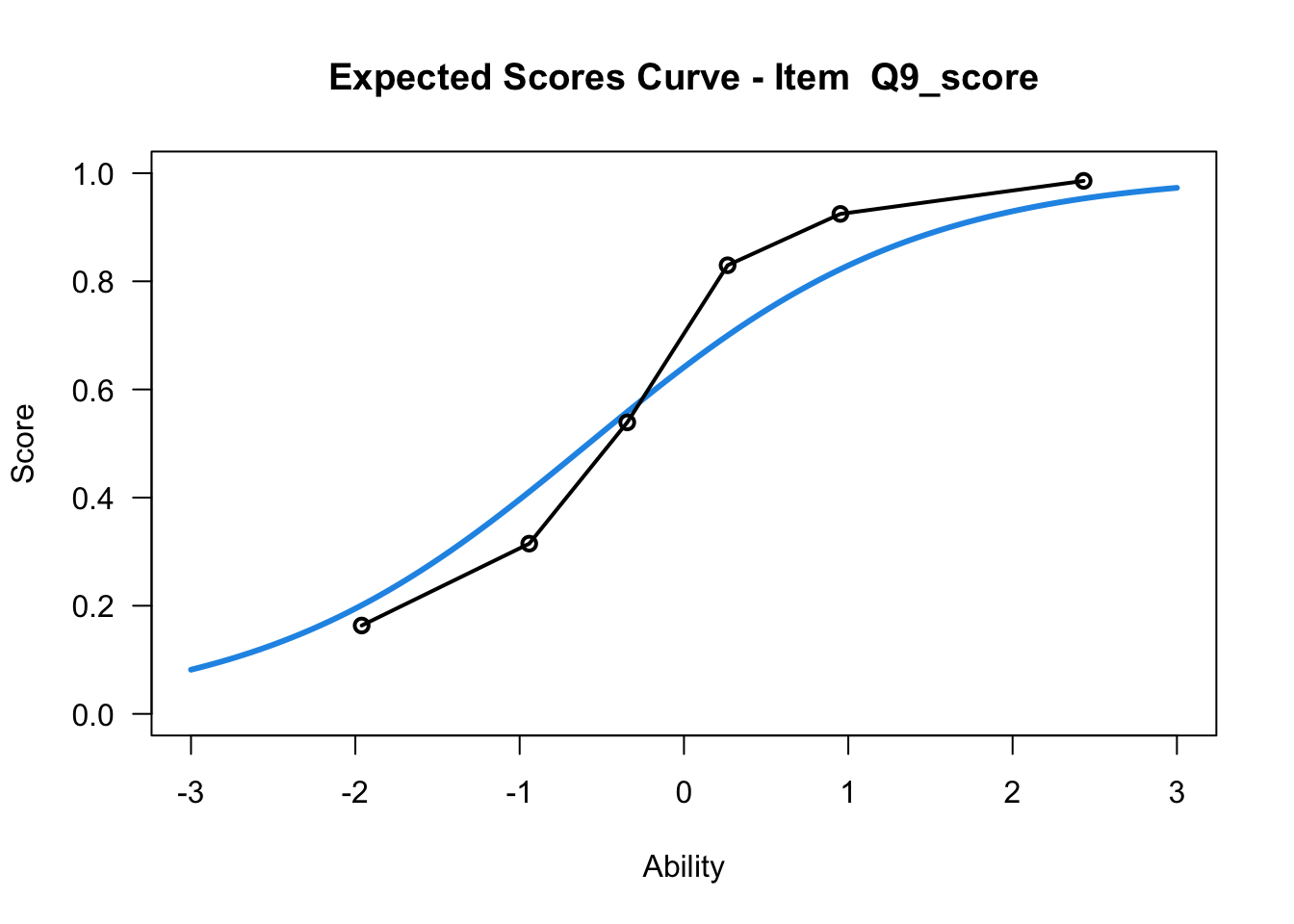
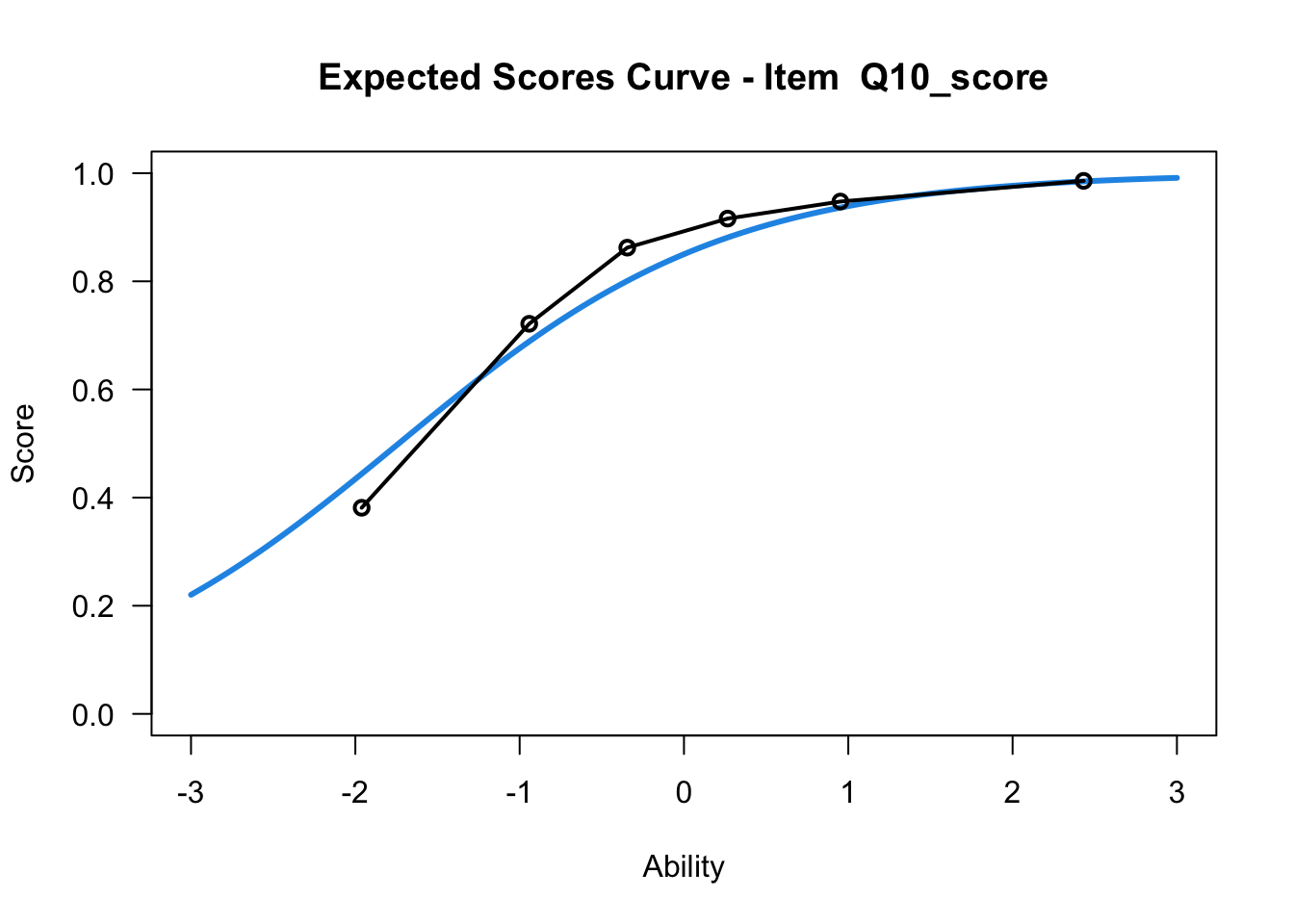
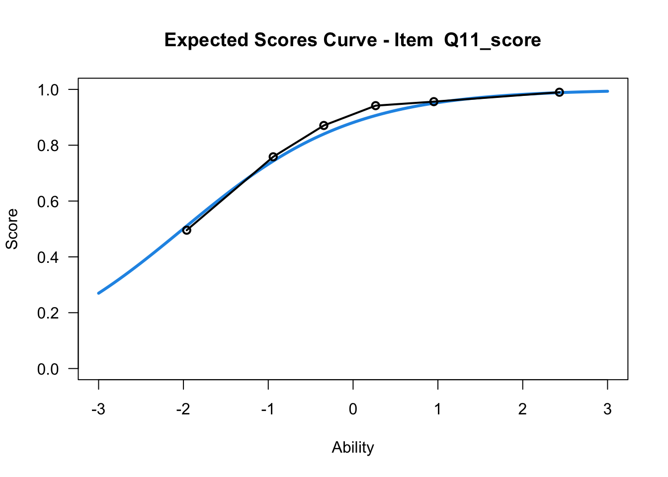
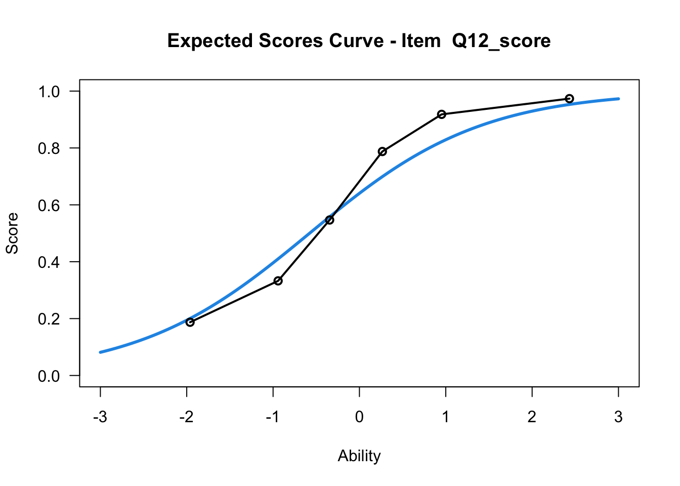
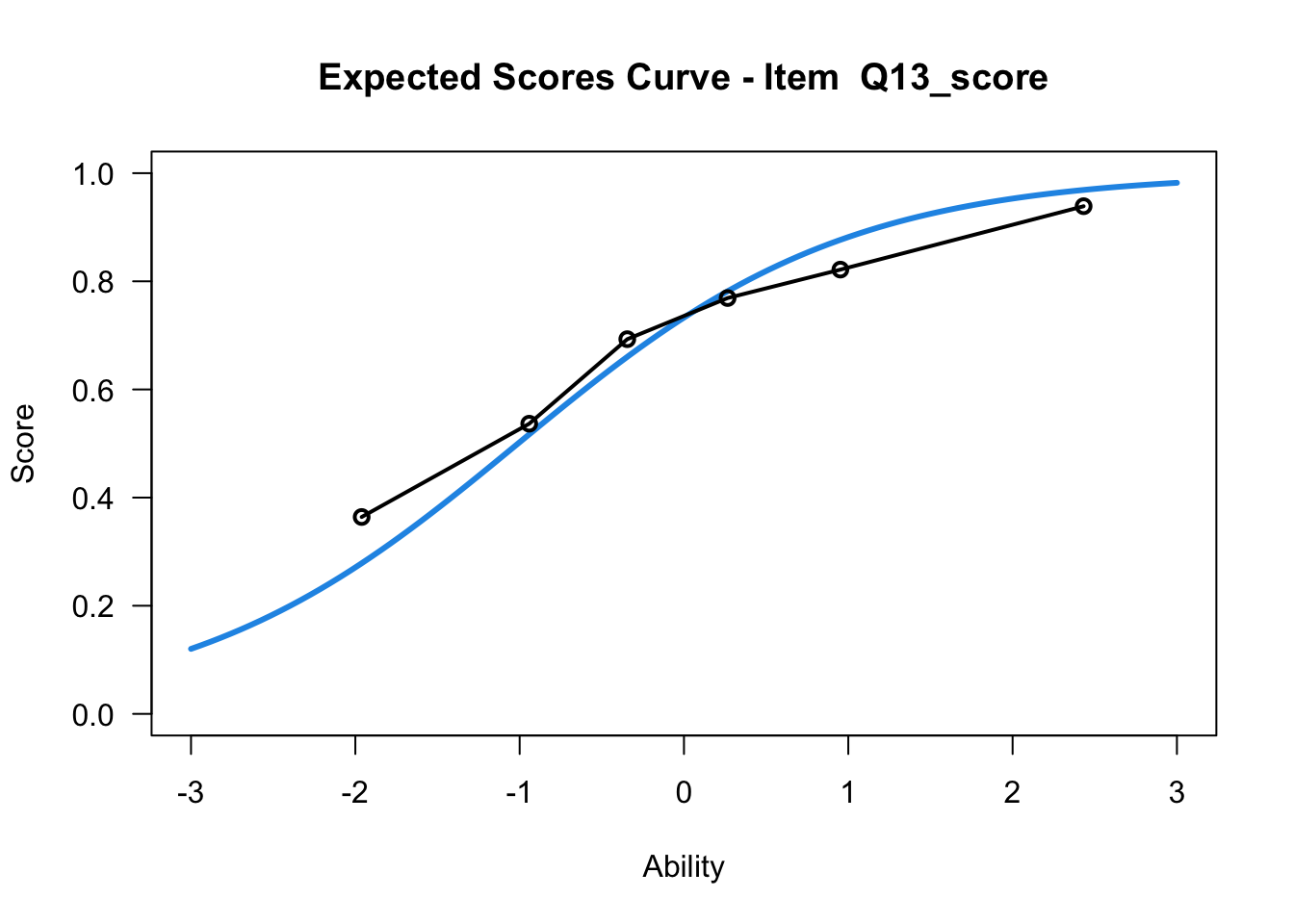
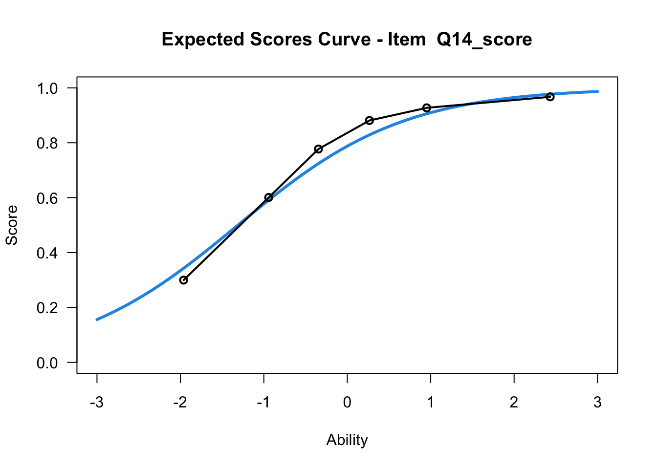
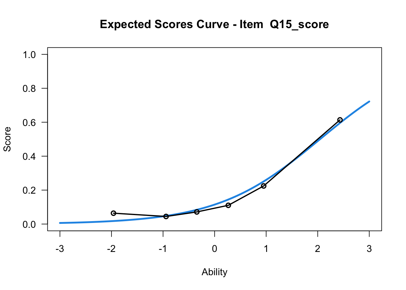
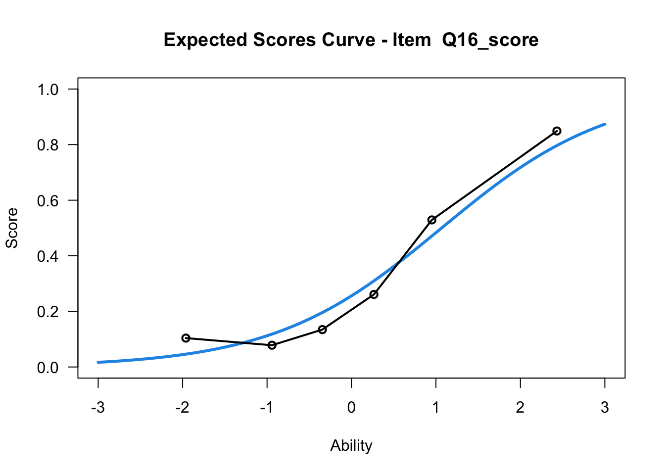
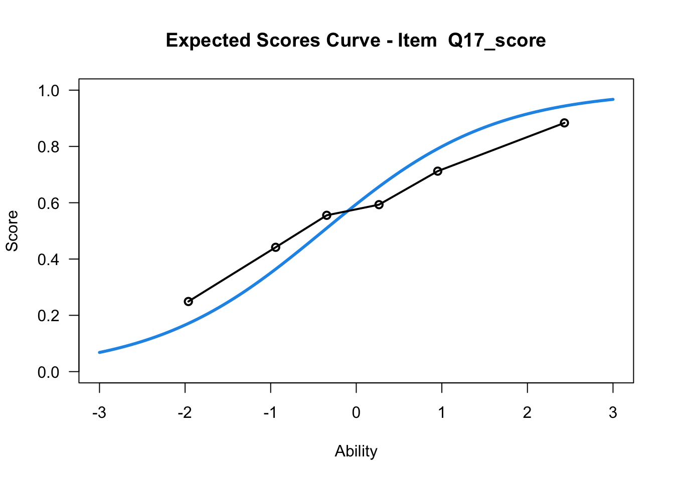
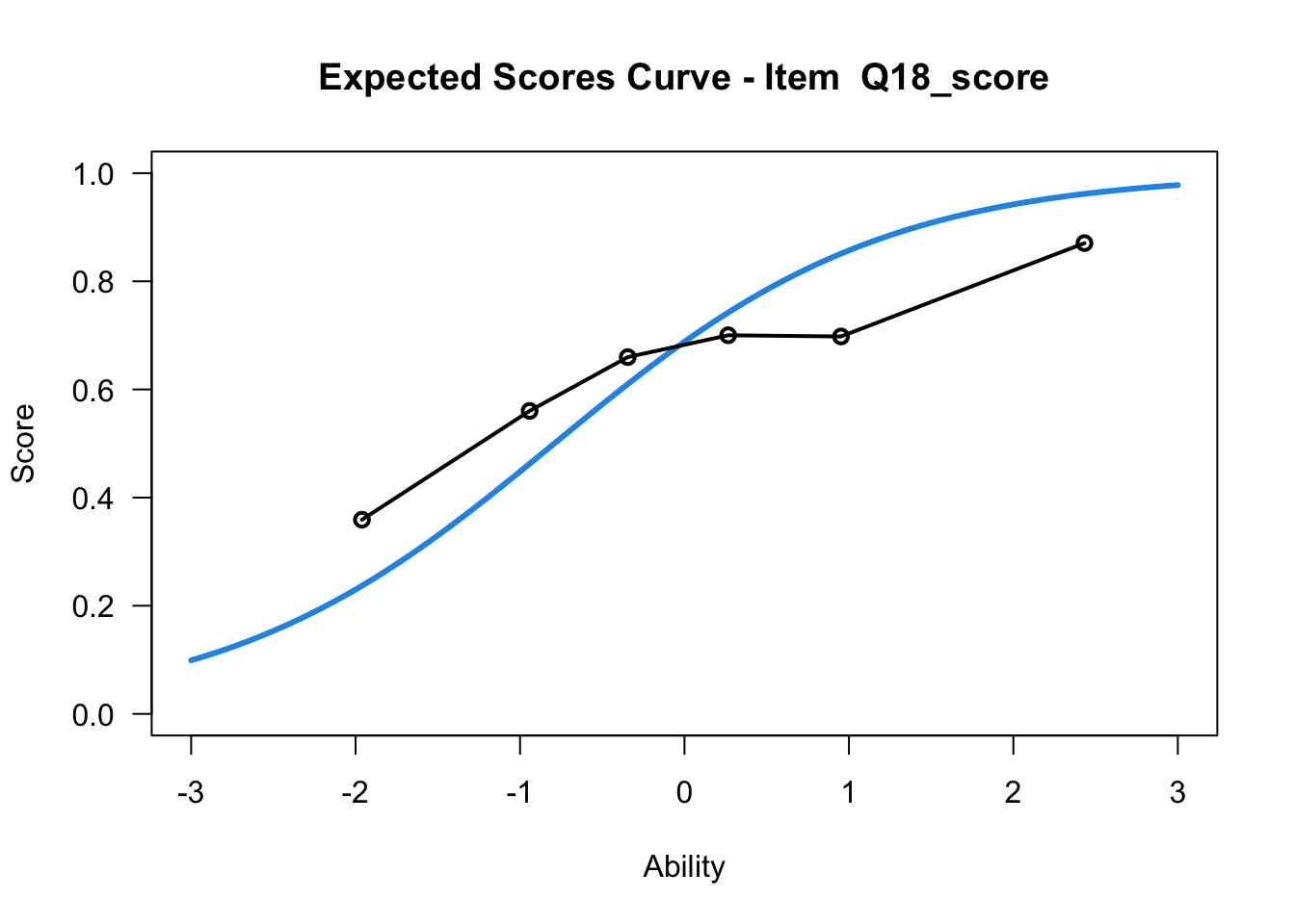
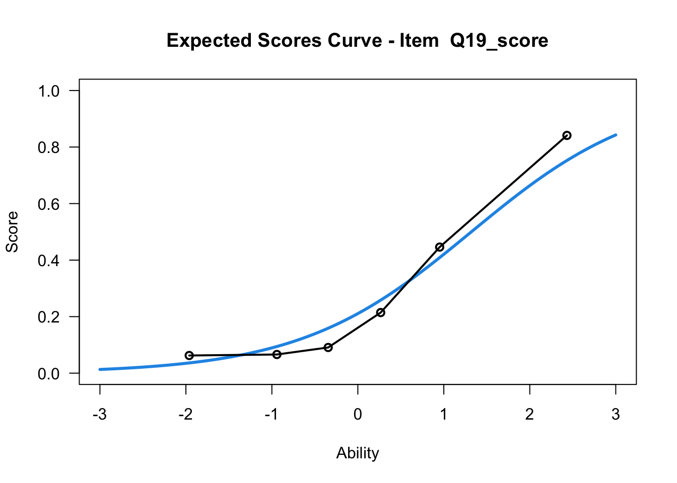
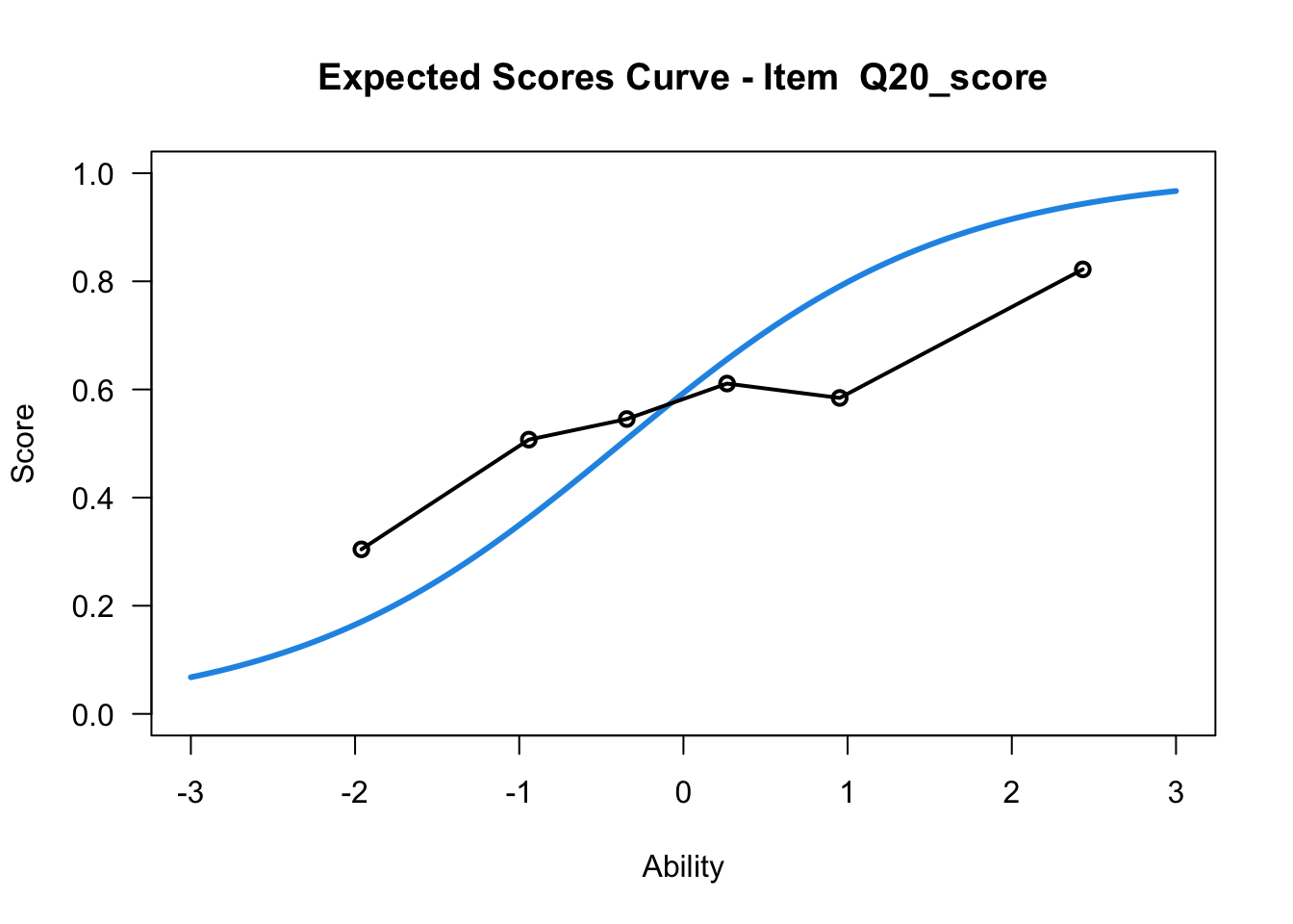
 Plots exported in png format into folder:
 /Users/chris/Documents/CM3/Plots

18.4 Item person map

library(WrightMap)
wrightMap(mod1$WLE, mod1$xsi, item.side = itemClassic)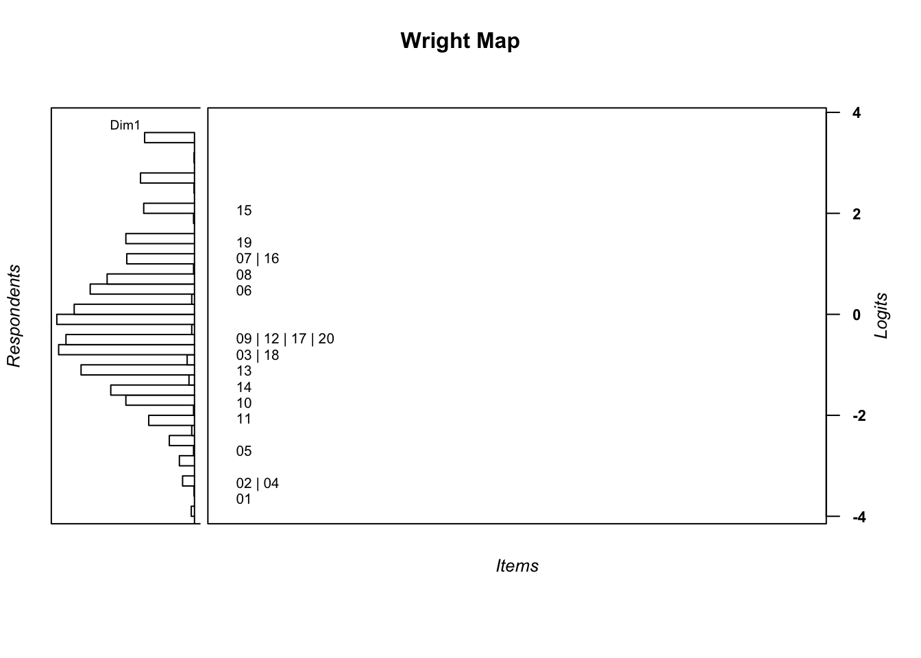

            [,1]
 [1,] -3.5930417
 [2,] -3.2171598
 [3,] -0.9719756
 [4,] -3.3412293
 [5,] -2.7708206
 [6,]  0.5110808
 [7,]  0.9973315
 [8,]  0.8525812
 [9,] -0.5805110
[10,] -1.7360466
[11,] -2.0044733
[12,] -0.5775793
[13,] -1.0096993
[14,] -1.3107828
[15,]  2.0443527
[16,]  1.0671544
[17,] -0.3840117
[18,] -0.7917916
[19,]  1.3204475
[20,] -0.3781141

18.5 Exercises

1. Compare IRT estimated item difficulties with CTT item scores.
2. Use the R function cor to calculate correlation. Use plot to show the relationship graphically.
3. Compare IRT reliability and CTT reliability
4. Visually compare ‘steepness’ of IRT observed ICC with CTT point-biserial correlation.
5. Compare students’ IRT ability measures (WLE) with students’ test scores (CTT).
6. Compute correlation and plot the two variables to show the relationship.

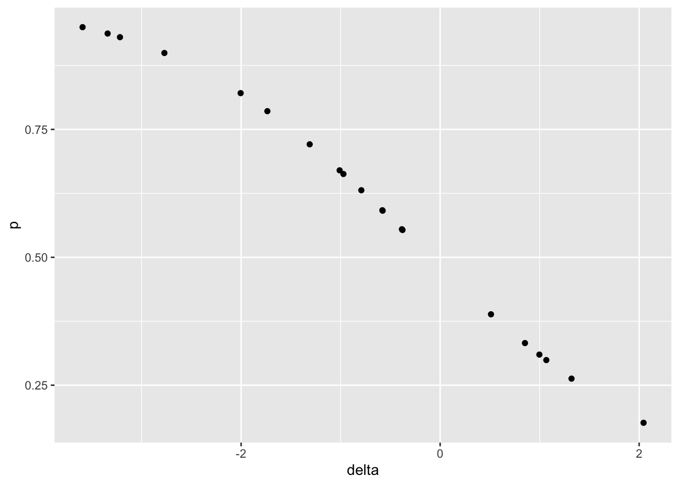
item_stats <- tibble(item = mod1$item$item, delta = mod1$item$xsi.item, p = mod1$item$M)
cor(item_stats$delta, item_stats$p)

[1] -0.9909958

p <- ggplot(item_stats, aes(x=delta, y=p))
p <- p + geom_point()
print (p)

Andrich, David, and Ida Marais. 2019. “The Idea of Measurement.” In A Course in Rasch Measurement Theory, 3–11. Springer Nature Singapore. https://doi.org/10.1007/978-981-13-7496-8_1.

Bond, Trevor G., Zi Yan, and Moritz Heene. 2020. Applying the Rasch Model: Fundamental Measurement in the Human Sciences. Routledge. https://doi.org/10.4324/9780429030499.

Cappelleri, Jason Lundy, J. C. 2014. “Overview of Classical Test Theory and Item Response Theory for the Quantitative Assessment of Items in Developing Patient-Reported Outcomes Measures.” Clinical Therapeutics 36 (5): 648–62. https://doi.org/https://doi.org/10.1016/j.clinthera.2014.04.006.

Cronbach, Lee J. 1951. “Coefficient Alpha and the Internal Structure of Tests.” Psychometrika 16 (3): 297–334. https://doi.org/10.1007/bf02310555.

Goldstein, H., and Steve Blinkhorn. 1982. “The Rasch Model Still Does Not Fit.” British Educational Research Journal 8 (2): 167–70. https://doi.org/10.1080/0141192820080207.

Lord, Frederic M, and Melvin R Novick. 2008. Statistical Theories of Mental Test Scores. IAP.

McNeish, Daniel. 2018. “Thanks Coefficient Alpha, We’ll Take It from Here.” Psychological Methods 23 (3): 412–33. https://doi.org/10.1037/met0000144.

Panayides, Panayiotis, Colin Robinson, and Peter Tymms. 2010. “The Assessment Revolution That Has Passed England by: Rasch Measurement.” British Educational Research Journal 36 (4): 611–26. https://doi.org/10.1080/01411920903018182.

Robitzsch, Alexander, Thomas Kiefer, and Margaret Wu. 2022. TAM: Test Analysis Modules. https://CRAN.R-project.org/package=TAM.

Sijtsma, Klaas. 2008. “On the Use, the Misuse, and the Very Limited Usefulness of Cronbach’s Alpha.” Psychometrika 74 (1): 107–20. https://doi.org/10.1007/s11336-008-9101-0.

Wright, Benjamin D, and Magdalena Mok. 2000. “Rasch Models Overview.” Journal of Applied Measurement 1 (1): 83–106.